
1
Danny Bragonier
Senior Project
Adviser: Dr. Smidt
California State Polytechnic University
Spring 2010
Statistical Analysis of Texas Holdem Poker

Page 2
Table of contents
• Overview
o Objective
o Abstract
o Background
• Introduction
o Explanation of Texas Holdem
o Glossary of terms
o Restriction of Analysis
• Univariate Analysis
o Data qualifications and parameters
o Analysis by hands
o Analysis by sessions
o Analysis by table sessions
o Analysis by stakes
• Regression Analysis
o Simple regression
o Multiple Regression
o Multiple Regression for NL 400
o Poker Tracker Analysis
• ANOVA Analysis
• Logistic Regression Analysis
• Outlier Analysis
• Conclusion
o Suggestions for Mike
o Overview
o What I learned

Page 3
Overview
Objective
Use statistical analysis to determine maximum profit potential for Mike Linn’s online
poker games.
Abstract
Gathered lifetime online Poker data for Mike Linn. Attempted to analyze data to obtain
information to maximize profit. Techniques included Univariate Analysis, Regression
analysis, Anova analysis, Logistic Regression, and outlier Analysis. After the analysis,
nothing of supreme importance or sustenance was found. Encountered issues with too much
power. Results lead to plenty of statistical significance, but little practical significance.
Results showed that the data did not provide all the answers that were being sought after, but
there was some value in examining the data in a strict statistical manner.
Background
My roommate, Mike Linn, is a professional online poker player. He has had success
profiting off less skilled players. I have spent many hours watching him play online and have
learned some of the things that make him successful and others not. I have often wondered
if there was a way to use my statistical analysis skills to quantify what things separate
winning players from losing players. Linn plays primarily online; consequently, there is an
abundance of data available to analyze. Linn has played and cashed in some live
tournaments (including placing 81
st
in the main event of the World Series of Poker). For the
purpose of this report we will only analyze his online play. When Mike sits down at his
computer to play poker he generally opens six to eighteen tables and plays anywhere from
thirty minutes to three hours. This will be referred to as a poker session. I will be doing the
bulk of my analysis on a session by session basis. Sometimes Linn ends his session with
more money than he started and sometimes not. As we know there is a fair bit of luck in
poker but the winning players win in the long run not because of luck but because of their
actions. The purpose of this report is to quantify what the actions Mike Linn takes to be a
winning player.
Introduction
Mike plays online poker primarily on the site Poker Stars. His screen name on Poker
Stars is Poly_Baller. Poker Stars (PS from now on) is required by law to record every hand
they host. They record each hand using something called a hand history file. The hand
history file is a text file that includes a comprehensive listing of everything that occurs at the
online poker table for each hand. Here is an example of one hand recorded in the hand
history.
Page 4
EXAMPLE
Hand #20306
PokerStars Game #18467389778: Hold'em No Limit ($2/$4 USD) - 2008/06/29 15:44:31 ET
Table 'Klonios II' 6-max Seat #5 is the button
Seat 1: Huge Gloves ($103.25 in chips)
Seat 2: FastEddie267 ($394 in chips)
Seat 3: UffzBrasche ($216.10 in chips)
Seat 4: KKozhuKK ($709.15 in chips)
Seat 5: Poly_Baller ($867.65 in chips)
Seat 6: cdeez8 ($432 in chips)
cdeez8: posts small blind $2
Huge Gloves: posts big blind $4
*** HOLE CARDS ***
Dealt to Poly_Baller [3c 3d]
FastEddie267: folds
UffzBrasche: calls $4
KKozhuKK: raises $10 to $14
Poly_Baller: calls $14
cdeez8: folds
Huge Gloves: folds
UffzBrasche: calls $10
*** FLOP *** [As 3s Tc]
UffzBrasche: bets $4
KKozhuKK: raises $32 to $36
Poly_Baller: calls $36
UffzBrasche: calls $32
*** TURN *** [As 3s Tc] [Kc]
UffzBrasche: bets $4
KKozhuKK: raises $36 to $40
Poly_Baller: calls $40
UffzBrasche: calls $36
*** RIVER *** [As 3s Tc Kc] [6h]
UffzBrasche: bets $4
KKozhuKK: raises $196 to $200
Poly_Baller: calls $200
UffzBrasche: calls $122.10 and is all-in
*** SHOW DOWN ***
KKozhuKK: shows [Td Ad] (two pair, Aces and Tens)
Poly_Baller: shows [3c 3d] (three of a kind, Threes)
Poly_Baller collected $147.80 from side pot
UffzBrasche: mucks hand
Poly_Baller collected $651.30 from main pot
KKozhuKK said, "f***in a joke honestly"
*** SUMMARY ***
Page 5
Total pot $802.10 Main pot $651.30. Side pot $147.80. | Rake $3
Board [As 3s Tc Kc 6h]
Seat 1: Huge Gloves (big blind) folded before Flop
Seat 2: FastEddie267 folded before Flop (didn't bet)
Seat 3: UffzBrasche mucked [4s Ac]
Seat 4: KKozhuKK showed [Td Ad] and lost with two pair, Aces and Tens
Seat 5: Poly_Baller (button) showed [3c 3d] and won ($799.10) with three of a kind, Threes
Seat 6: cdeez8 (small blind) folded before Flop
When I emailed PS they emailed me back with 24 .zip files. After unzipping the files
they revealed 24 massive .txt files. There were 24 files because PS had Poly_Ballers hand
histories on 24 different servers. Recently people have developed ways to read in these
hand histories and convert them into poker data. The leading poker analysis software is
called Poker Manager. I used this program to import all the hand histories that PS provided
me. After taking an initial look at the data it was clear that the data were not complete. I may
not have realized this if the month of February 2009 was not missing. This happened to be
one of Mike’s best months ever and there was simply no data on it. I emailed PS again and
luckily they have very good customer service. They said they had made a mistake and there
should in fact be 28 files instead of 24. I imported the new 28 text files and I believe these to
be a complete representation of Poly_Ballers online poker play on PS. The 28 .txt files will
be provided along with this report.
Explanation of No limit Texas Holdem Poker
To begin, anywhere from 2 to 10 players sit around a circular table. Before cards are
dealt the forced bets must be paid, which are called the big blind and the little blind. The
player one seat to the left of the dealer places the small blind. The player one seat to the left
of the little blind places the big blind. The dealer will then deal two cards to each player face
down. These are known as the pocket cards or hole cards. Each player must then decide if
they wish to call the current bet (the big blind, which is the highest amount bet at this point)
which means to match it, fold their hand without betting if they don't like their cards, or raise
the bet by putting more money into the pot. Each player, starting with the seat to the left of
the big blind, makes their choice and acts. If a player raises the bet, each player must now
call the new amount, including those who may have already acted. At any time a player may
re-raise, meaning that they raise it again beyond the amount it was raised previously. Once
there are no more raises and everyone has acted the dealer will deal the flop. The flop is
three cards placed face up in the middle of the table. These are the first community cards.
Each player can use their two hole cards in conjunction with the three flop cards to make the
best 5 card hand. The first player to the left of the dealer that is still in the hand is the first to
act. They have the option to check or bet. Checking is defined as not committing any more
money to the pot and continuing on to the next player. After everyone has had their chance
to act, the dealer will deal another community card. This is known as the turn. Betting is
done exactly the same as on the flop. After everyone has had their turn to act, the final card
is dealt. This is known as the river. The collection of the five community cards is known as
the board. There is a final round of betting. Anyone still in the hand is now at showdown.
The player that can make the best 5 card hand will win the pot. Each player has the option to
Page 6
use zero, one, or both of their hole cards to make the best 5 card hand. This means if there
are four spades on the board and I hold one spade in my hand I can play a flush. Since this
is no limit Texas Holdem each player has the option to go wager all their chips and go all in
at any time.
Glossary of terms
Poker has its own jargon that could be take many, many pages to explain. Below is a
listing of the technical terms needed for this report.
Game Type – defined by the small and big blind of the limit being played. Also referred to by
the maximum buy in. The max buy in is usually 100 times the big blind. e.g. no limit holdem
with small blind of 2 and big blind 4 is referred to NL 400.
NL-No limit means a player can wager all his chips at any time during the hand
LIM- Players can only bet certain amounts on different streets that are proportional to the
blinds.
EV-This is calculated by taking the actual amount won and either deducting or adding the
amount you would have won with average luck.
Hands- Total number of hands played at the level specified.
$- Money won or lost at that limit. Loses documented in red and parentheses.
BB/100- Amount of Big Bets won per 100 hands. A Big Bet is defined by twice the big blind.
VPIP%- Voluntarily put money in pot percentage. This is a measure of how loose or tight a
player is. VP$IP is expressed as a percentage of the time a player puts money into a pot to
see a flop in Hold'em. The big blind is not considered voluntary, so if a player checks his big
blind, that is not considered in the VP$IP calculation. However, if the big blind calls a raise,
then it is considered for VPIP. If a player calls or raises only to fold to a further pre-flop raise,
this also counts for VPIP%.
PFR%-PreFlop Raises. This is a measure of pre flop aggression. Simply, the percent of time
a player raises before the flop.
3bet%-Percentage of time player 3 bets. A 3 bet is defined by the player betting, getting
raised, and then the player reraising.
WTSD%- Went to Show Down. This is a measurement of how willing a player is to stay in
the hand until the end. Simply computed as number of hands showed down divided by
hands played.
W$SD%- Percentage of time a player has money at show down. This can be used as a
measure of how often a player bluffs.
Agg-This is the aggression factor. This is the aggressive actions divided by calls. This is
found by adding total number of bets and raises and dividing by number of calls.
Agg%-This is the aggression frequency. This is often referred to as the best way to assess a
player’s aggression. It is found by [Times Raised + Times Bet] / [Times Raised + Times Bet
+ Times Called + Times Folded]. The higher the percentage the more likely the player is
bluffing more hands.

Page 7
Restriction of Analysis
I should mention that the analysis that follows in the rest of the report is for the most
part inferential. However, the data I have is from a population and is not a random sample. If
we can see the data as a “sample” of lifetime data then there is no issue. It is important to
remember we are dealing with population data and not a random sample when making
predictions, extrapolation and inference.
Univariate Analysis
Univariate reports are used to get a better idea of what the data looks like simply.
Data qualifications and parameters
For the purpose of this project I will only be analyzing data that was obtained between
March 31, 2006 and Jan 15, 2010. In that span we have data on 2,178,217 hands. Mike is
primarily a Texas Holdem player; however, he has played some Omaha. Omaha is a
variant of Texas holdem. I decided to only analyze the holdem hands. The style in
which one plays Omaha and holdem are completely different. Their winning strategies
have many differences. I thought it would be more appropriate to only analyze Mike’s
holdem play. After removing all the Omaha hands there were now only 1,883,932
hands.
Univariate analysis by hands
Throughout this report the primary response variable is going to be profit. Below
in figure 1 is a time series graph provided by poker manager that shows every holdem
hand played versus profit.

Page 8
Figure 1
Figure 1 is essentially a time series graph with hands on the x-axis and profit on the y-
axis
As you can see there are many up and down swings in the graph. My aim to try
and figure out what makes the graph go up and down but more importantly, why it has a
general upward trend.
Univariate analysis by Sessions
I initially thought that the bulk of my analysis would be based on sessions. These
sessions were defined as Mike opening up a group of tables and playing for a period of
time then closing all the tables. My initial thought would be that profit would be response
variable. However, it became clear that using just profit would not be sufficient. If Mike
won a 400 dollar pot while playing no limit 400 then it means we did well to get the entire
chip stack of another player. However, if he is playing NL 5000 and he wins 400, then it
means he won a very small pot and may not have had to play as well as he did at NL
400. Because of this fact it makes a lot more sense to look at a standardized version of
profit. The most logical is BB/100. This will also be referred to as win rate. I could not
develop a win rate variable for the session’s data because he would often play different
stakes during the same session. He might be playing 5 tables of NL 400 and 4 tables of
NL 1000. This makes it impossible to convert profit to win rate. Thus, I had to break

Page 9
each session down to each table and look at the data that way. Regardless, figure 2
shows the univariate stats for sessions.
Figure 2
Figure 2 shows that the means for each variable match very closely to the means in figure 3.
Also Bin profit shows that Mike won 61.67% of his sessions.
Univariate Analysis by Table Sessions
After looking at initial reports of the data it was clear that I would have to clean it up
before it was usable. The first thing that became clear was that there were insanely large
outliers in nearly every variable. In figure 4 you can see all the outliers in each of the
variables. The reason for all these outliers is that some of these sessions are only a few
hands long. This small sample size of hands is making the variance very high. My aim was
to lower the variance by only including sessions that contained more than a certain number of
hands. I was unsure what an acceptable number to use was. I examined the sessions with
only more than 25, 50, 75, and 100 hands. Because of the nature of the data an interesting
thing happened. When I was only looking at sessions with more than 100 hands I had lost
well over half the data in terms of sessions. There are 19069 sessions total and only 7698
sessions with more than 100 hands. However, there are 1.88 million total hands and about
1.3 million are included in the sessions with over 100 hands. Also, in my attempt to raise
sample size by only including sessions with a substantial amount of hands I was actually
lowering the sample size of number of sessions. Another very interesting thing happened
when I was only analyzing sessions with more than 100 hands. Mike was actually a losing
player. His profit was a negative
157,000 dollars. That means in sessions with less than 100
hands he was positive almost
300,000 dollars. This was a very promising result for my
regression analysis to come. Another thing that caught my eye was that even though Mike
was in the red 157 thousand dollars his win rate (i.e. BB/100) was still positive at
2.41. What
this means to me is that for longer sessions Mike suffers great losses at higher stakes but
can still win consistently at lower stakes to counteract those huge losing sessions. Since I
would be looking at win rate and not straight profit I knew when I would run my regression

Page 10
analysis my coefficient for hands would not be as negative since the win rate only went from
6.63 to 2.41. After examining the scatter plots in figure 3 I decided I would do all my session
analysis on sessions that lasted longer than 50 hands. I made this decision because the
scatter plot showed no substantial outliers and eliminated the least amount of data. It
became clear after examining these scatter plots I was going to have a problem with constant
variance for the residuals. I know that we are not supposed to just throw away data just
because it is an outlier. However, with less than 50 hands the data is too dependent on the
cards Mike is receiving and not on his playing style.
Figure 3 Figure 3 cont.
Figure 3 shows the differences in basic
statistics when we remove different
amounts of the data. The data does not
change much when all of it is present
and when the sessions with less than
50 hands are removed.
Page 11
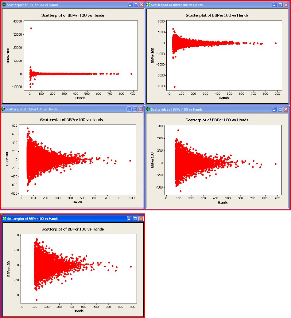
Figure 4
Figure 4 shows how we can get rid of the
crazy outliers when we remove the short
sessions. Top left has all the data, top right
does not contain sessions with less than 25
hands, middle left contains sessions with
more than 50 hands, then 75 hands, then
100 hands in bottom left.

Page 12
The top left scatter plot shows hands vs. bbper100. It shows that there is a tremendous
amount of variance when we include all the data, standard deviation=342. The next scatter
plot (top right) has sessions with less than 25 hands removed. You can see that the variance
is better but still not very good, standard deviation=141. The next three scatter plots have
less than 50, 75, and 100 hand sessions removed. The variance does not improve
significantly from 50 to 100, standard deviation goes from 119 to 99. This is why I decided to
use 50 hands as my cut off. Even with removing the short sessions it is clear we are going to
have issues with unequal variance.
Figure 5, figure 6, and Figure 7 show basic histograms of the explanatory variables we will be
dealing with in the analysis
Figure 5
As you can see, hands is skewed right. Mike plays the bulk of his sessions with less
than 200 hands. Profit per hour and profit look very similar. It appears they are symmetric
around zero and bell shaped with some very large outliers on both sides. The minutes
played group looks similar to hands, as it should. It looks like the bulk of Mike’s sessions last
about an hour.

Page 13
Figure 6
The histograms for PFR% and VPIP% look quite similar. PFR% is centered around
20% as VPIP% is centered around 30%. EV looks like it is symmetric about zero and has
some very large outliers on both sides. Average players histogram shows that Mike mostly
plays at 6 person maximum tables that usually table 5 players.

Page 14
Figure 7
W$SD is a very interesting histogram. It ranges all the way from zero to one hundred.
There is a substantial amount of data that is at the extremes as well. The 3 bet % is skewed
right and never really gets above 25%. WTSD% is fairly normal and symmetric about 28%.
Aggression factor is also skewed right and centered around 6.

Page 15
Figure 8 below shows the histogram for our response variable
Figure 8
The above figure is my response variable. The histogram shows that the data is looking
quite nice, perhaps even normal. After looking at a normal probability plot in Figure 9 it
shows that although the data is symmetrical and bell shaped it is not normal.
Figure 9
There are actually 95% CI
limits on Figure 9. However, since
there is so much data they are very
close to the normal line and barely
visible. When we have such a
large amount of data perfect
normality is nearly impossible.
Based on the histogram the data is
behaving quite normally. Most
statisticians would be very satisfied
with the normality in Figure 8 given
the sample size

Page 16
Univariate analysis by Stakes
Below in Figure 10 is a chart that shows all the stats differentiated by the different
stakes that Mike has played.
Figure 10
Figure 10 shows a breakdown of each variable by what stake Mike is playing.
It is clear from Figure 10 that the best stake in terms of profit in NL 400 and his worst
is NL 5000. Mike has also played the most hands at 2/4. There will be more in depth
analysis on the impact of stakes in the ANOVA section of the report, page 35.
Regression Analysis
~As stated previously~
I thought the best way to start this analysis would be to look at it on a session-by-
session basis. I thought there would be certain variables that would contribute to a winning
or losing session. There are certain styles of play that often result in profit. I think that the
variables I included can capture the different styles of play. For this portion of my analysis I
am going to use dollars per 100 big blinds as my response. This is a way to standardize
winnings. Since Mike plays many different stakes it makes the most sense to look at profit as
a percentage of the big blind. The first problem I ran into with this approach was that

Page 17
sometimes Mike played different stakes during the same session. This would make it
impossible to develop a bb/100 response variable. Luckily, Poker Manager is able to
generate a .csv file that is partitioned by each individual table’s session. I did the bulk of the
analysis on this data frame.
Simple Regression
The first variable that I did regression analysis on was hands per session. My
hypothesis was that the longer Mike played the worse he would perform. This is where I ran
into my first problem. Below in Figure 11 is the four in one graph of the residuals generated
by this regression analysis.
Figure 11
The top right graph in Figure 11 shows a huge problem with unequal variance of the
residuals
In figure 11 above it is clear that there is a problem with the residuals vs fits. The
residuals are also apparently not normal based on the normal probability plots, despite the
histogram looking symmetric. This is significantly less of an issue considering the sample
size. In an ill-fated attempt to fix the unequal variance and the problem with normality I tried
some transformations. My first transformation attempted was to log the response. In order to
do this I had to take the log of the absolute value of the bb/100 then get the negative sign
back where it was needed. Figure 12 shows the residual plots.

Page 18
Figure 12
Figure 12 shows the transformation clearly did not work.
The next thought was to transform the X variable, by logging hands. Figure 13 is the residual
analysis.

Page 19
Figure 13
Also an unsuccessful transformation shown in Figure 13
This also did not work. I tried every combination of natural logs, square roots,
squaring and different powers. I could not obtain any combination of transformations that
helped the residuals. The remarkable thing I noticed during these transforms was that no
matter what I did the variable hands stayed significant. Below in Figure 14 is the output that
shows the original regression results.
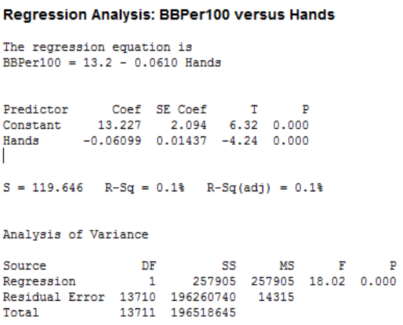
Page 20
Figure 14
Output for simple regression analysis
Disappointingly, the R-squared value is essentially zero. It seems (based on this
invalid analysis) that the length of the session does not explain any of the variance in Mike’s
win rate. However, as I suspected, the coefficient is negative and statistically significant.
Since the sample size is so large it seems that no matter what variable is being used to
predict bb/100, it will be a significant predictor. This was the first indication that there would
be plenty of statistical significance but little practical significance. With sample sizes as large
as I had, the power of each test was immense.
More simple regression
I decided to take a look at each of the explanatory variables as a single predictor for
win rate. The variable W$SD looked the most promising. Figure 15 shows the residual
analysis.

Page 21
Figure 15
These are much more promising residuals. There is some pattern in the residuals vs. fits
however it is not that bad. The histogram of residuals looks very symmetric and normal. The
normal probability does not look that bad even though there is a very small P-value
suggesting non-normality. With these large sample sizes we almost never see perfect
normality.

Page 22
Figure 16 shows the output from Minitab on the regression analysis.
Figure 16
The intercept is interpretable in this case and it is significant. If mike does not win any
money at showdown he can expect an average win rate of -108. This is a significant loss.
As such, the coefficient for W$SD is quite positive and very significant. The corresponding t-
value is a high 73.84 leading to an incredibly small P-value. The R-squared value is 28.5%,
which is not great but promising for only one predictor. This is certainly an upgrade from .1%
from the previous simple regression analysis.
Below in Figure 17 is a matrix plot for all the variables of interest. You can see that
W$SD clearly has the best linear association with win rate.

Page 23
Figure 17
You can see that none of the other predictors had strong linear associations with
BB/100. However there were some instances of association between certain explanatory
variables. The strongest correlation, based on the correlation matrix in Figure 18, was
between minutes played and hands. The Pearson correlation being .94 is not surprising.
PFR% and VPIP% also had a high Pearson correlation of .837. This is also expected
because a PFR is considered as volunteering money in the pot.
Figure 18

Page 24
Multiple Regression Analysis
Now, with the simple regression complete I can begin the multiple regression. I am going to
start with the saturated model. Below is the analysis. Figure 19 shows the residual analysis.

Page 25
Figure 19
Residual vs. fits shows some issues but there are only a few points that do not behave.
The residual plots carry the same story as previously. They are not the best but they
are acceptable considering the sample size and I am going to continue the analysis. There
are only a few observations that are making the residual vs. fits graph look imperfect. This is
acceptable.

Page 26
Below, Figure 20 is the Minitab output for the saturated model.
Figure 20
This is the first time in my report that I realized that it would not be acceptable to
include EV as an explanatory variable. Poker Manager calculates EV as a function of profit.
It takes the actual expected values (as statisticians know the term) and then takes the
difference of that number and the actual profit earned. This does not work for my analysis
because then I have the problem of predicting BB/100 (which is a function of profit) with EV,
which is also a function of profit. Thus, I will not be using EV for the rest of my analysis.
Figure 22 shows the new saturated model without EV. While Figure 21 shows the residual
analysis.

Page 27
Figure 21
Residual plots actually look a little better without EV in the model.

Page 28
Figure 22
The first thing to notice is that the R-Squared value went down a lot. It turns out that
EV was accounting for a large amount of the variation in win rate. The new R-squared is not
even 1% higher than the model with only W%SD. Yet, 6 out of 10 predictors are significant
at the .05 level. The new R-squared value is about 30%. This was disappointing for me.
This means that there was still 70% of variation in win rate unaccounted for. I believe the
explanatory variables included are a fairly good representation of the skill accounted for
poker. Perhaps I am missing a key variable. Perhaps that variable is luck. The most
profound discovery I may have found in this report is that poker is 30% skill and 70% luck.
Poker analysts have not found a clear and exact way to quantify luck in poker without
knowing every players cards from the beginning of the hand. Although, every poker player
will tell you how unlucky they are.
I noticed that the two Betas that had the lowest t values and highest P-values were
also two of the variables that had the highest correlation. First, I took Minutes Played out first
since we have been speaking in terms of hands rather than time for most of this report. My
thought was that this would now make hands significant. However, Hands remained

Page 29
insignificant. So, I put Time played back in the model and took out Hands. Hands remained
significant. The model did not change in terms of residuals or R-squared adjusted.
Next, I took out rake. Rake had a high p-value. Again nothing happened. No change in R-
squared adjusted or residuals. None of the other variables coefficients’ or P-values’ changed
significantly. Next, I took out PFR%. This was not a variable I would suspect as being
insignificant. In the poker community it is often one of the most discussed statistics when
determining good play. Given the high p-value for PFR%, not surprisingly, things remained
the same after the removal.
Now there remained only one insignificant variable, VPIP%. I removed that variable
and arrived at my first multiple regression model. Seen below in Figure 23.
Figure 23
It seems the best regression equation I could find is:
BB/100 = 55 - .111 Minutes.Played – 6.8 Avg.Players - .526 3Bet% + 1.15 Agg.Factor - .397
WTSD% + 2.44 W$SD
The significant variables I found were Minutes played, average players, 3 bet %,
Aggression factor, WTSD% and W$SD. These variables were all statistically significant for
the regression analysis. However, the R sq. is quite low. I was hoping for a value closer to
80% when I started this project. The problem with having such a high sample size is that
almost any variable can be found to be statistically significant but few are practically
significant. If we compare this model with many predictors to the model with just W$SD we

Page 30
are only gaining about 1% of R-sq. This tells me that although the rest of the predictors are
statistically significantly different from zero they may not be practically significant.
I was curious to see if a partial F test would even say this was a substantially better
model from the simple regression with only W$SD.
Partial F-test
At least one differs from zero
F= 24.55
P-value ≈ 0
Reject the null hypothesis meaning the final multiple regression model is in fact adding
additional information. However, I am skeptical it added any practical value.

Page 31
Forward and backward stepwise selection yielded the same optimal model, seen in Figure
24.
Figure 24
Best subsets also shows that the model I found is optimal, based on the lowest Mallows Cp.
Shown in Figure 25. Every method I used to get from the saturated model to the final model
yielded the same significant variables. I am confident the final model I obtained is the best
model available.

Page 32
Figure 25
Multiple regression Analysis for NL400
I decided to do a multiple regression analysis on only one limit of play. Mike has
played the most hands, by far, at No limit 400. Mike has played 1226761 hands at this stake
and profited 229,460.75 dollars. This is also by the far the most profit he has made at any
stake. Like in the complete analysis I had to remove the sessions that were less than 50
hands. Below in Figure 26 is a scatter plot of hands Vs Win Rate, without any sessions with
less than 50 hands.

Page 33
Figure 26
9008007006005004003002001000
750
500
250
0
-250
-500
Hands
BBPer100
Scatterplot of BBPer100 vs Hands
Below is the saturated model residual analysis and results.
Figure 27
The residual analysis actually looks pretty good. There is a slight problem with
normality but nothing ghastly. Also, there seems to be a bit of an upward trend in the residual
vs fits graph but also nothing too terrible.

Page 34
Figure 28
The regression analysis looks similar to the saturated model that included every stake.
The R-squared are nearly identical, as are some of the coefficients. I came to the final model
in a similar approach as I performed with all the data. Figure 29 shows the final model.

Page 35
Figure 29
This analysis proved to be slightly different in terms of what variables are included in the
model. Figure 30 is a chart that illustrates the differences.
Figure 30
Variable All stakes NL 400
Minutes Played -.111 -.095
Average players -6.801 -10.069
3 bet% -.5264
VPIP% .7027
Aggression factor 1.1475 1.1442
PFR% -.8142
WTSD% -.39693 -.4618
W$SD 2.4408 2.39651
For the most part the coefficients are very similar for the overlapping explanatory
variables. The NL 400 model penalizes a bit more for more people at the table. The NL 400
model also has one more significant variable. The variables in both models that do not have
their counterpart in the other model are all small, meaning close to zero and more in the
model because of their statistical significant but not their practical significance.
Page 36
Poker Tracker Analysis
The output shown below in Figure 31 is from Pokertableratings.com or PTR. PTR is a
free online site that aims to track every player’s performance that plays online poker. It is
useful for quickly checking the statistics of opponents you meet online. It is effective for
getting a general idea of a player. There are drawbacks though. The site only has data for
the last year and a half, roughly. Also it tends to miss some sessions for whatever reason.
So, it is not perfect, but many players use it as a general guide to look at different player’s
playing style. The output below compares Mike’s play at NL 400 to other players at the same
stakes. It shows that mikes play is pretty average in terms of looseness but he is quite
aggressive compared to others. It also shows that his win rate is right in the middle of the y
axis maybe a bit higher than average. The bottom two graphs show his show down
frequency as being fairly average because his point is right at the peak. They do not
explicitly explain how they arrive at their scale for looseness and aggression but it seems to
be a composite of some of the variables I have included in my report.

Page 37
Figure 30

Page 38
ANOVA Analysis
I wanted to see if Mike played differently at different stakes. In theory, Mike should
play the same no matter what stakes he is playing. If it is a winning strategy at one level then
in theory it should work at other stakes because you are still playing the same game. The
first variable I wanted to test was his Win Rate. Figure 31 shows the 1-way ANOVA analysis.
Figure 30
Clearly, I need to remove the stakes where he has not played many sessions with
more than 50 hands. I decided to remove the stakes where Mike has played less than 50
sessions. Below is the new analysis.

Page 39
Figure 31
The output suggests that there is no difference in the mean win rates at each stake.
The next variable that I wanted to check was the aggression factor. Mike plays quite
aggressive compared to other players. Often one of the consequences of playing at higher
stakes is that players get timid, and thus not as aggressive. Below in Figure 32 is the
ANOVA analysis.

Page 40
Figure 32
Once again there is no difference in mean aggression factors across all stakes.
I found one significant ANOVA analysis that I did not expect to find. It turns out that
the number of people at the table has a significant difference. Analysis in Figure 33.

Page 41
Figure 33
It appears that at the highest stake, 25/50, Mike tended to play with more people.
This is interesting because in the regression analysis avg.Players was a significant predictor
with a negative coefficient. Also 25/50 is the only stake that Mike has a negative win rate.
Page 42
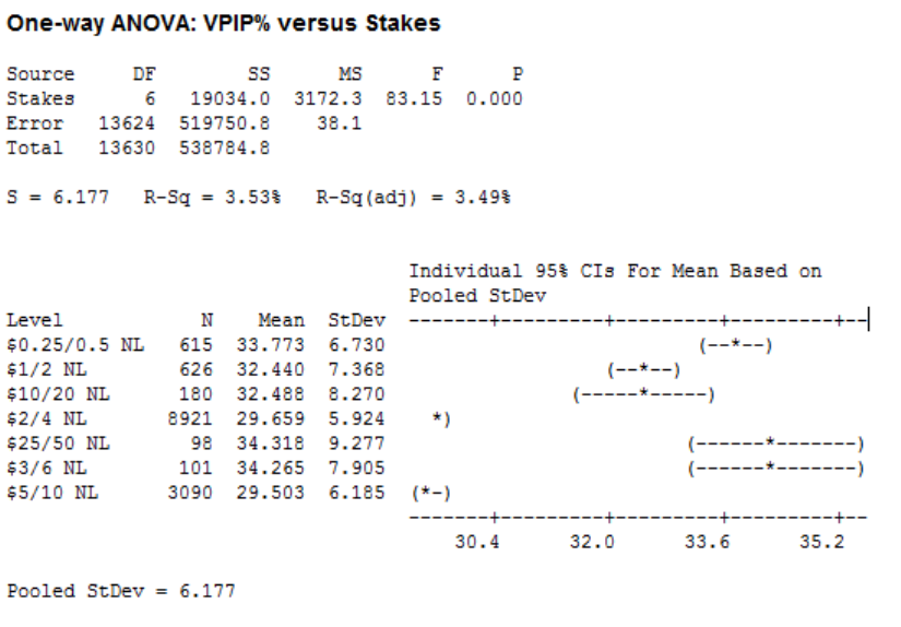
Figure 34
Figure 34 shows VPIP% had at least one significantly different mean at the different
stakes. It appears when Mike plays 2/4, his most profitable stake, he has a lower VPIP%.
This may be an indication that a lower VPIP% is better but the regression analysis showed
that it had a slightly positive slope. I wouldn’t say that the difference in means is only
statistically significant and not practically significant either. There is about a 4% difference in
the mean at 2/4 compared to the other group of means.

Page 43
Figure 35
The means for PFR% seem to be all over the place, each mean being different from
almost all the other means. The only thing that could be intelligible from this is that Mike has
the highest PFR% at 25/50 which is the highest stakes he played and his only stake where
he has a losing win rate.

Page 44
Figure 36
This ANOVA analysis may be a case of statistical significance but not practical significance.
The difference between the lowest and highest is only a little more than 2%.
Figure 37
Page 45
The same case here as above. There is only statistical significance but not practical
differences. The lowest mean is only 2 percent lower than the highest which is not much.
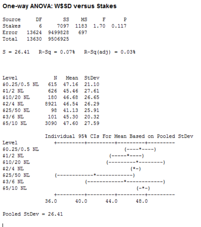
Figure 38
W$SD did not show any statistical differences in means. This was surprising since in
the last two analyses we had a problem with too much statistically significant evidence. If you
compare the standard deviations for W$SD to all the other explanatory variables you will see
that they are much higher for W$SD. This can be explained by looking at the histogram for
W$SD. Below in Figure 39 is a dot plot chart that shows that the distribution of W$SD looks
basically the same for each stake.

Page 46
Figure 39
Page 47
Logistic Regression Analysis
I thought it would be pertinent to analyze the session analysis using logistic
regression. This would allow me to look at whether or not certain aspects of Mike’s game
result in profit or loss. I would also be able to look at which variables contributed to increased
odds of success. I made the Profit variable dichotomous by assigning it a value of 1 if the
session resulted in any gains above zero dollars. Similarly, I assigned a zero to any losing
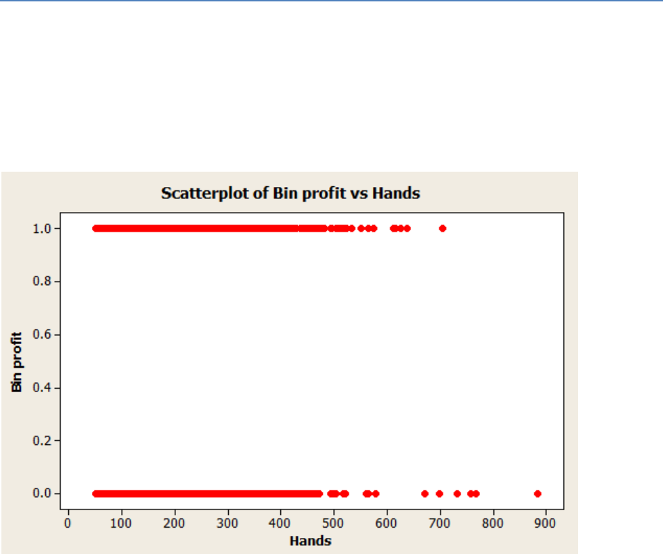
sessions. I started with simple logistic regression. The first model I fit was just using hands
as a predictor. Below is a scatter plot or hands vs the dichotomous profit variable.
The plot shows no real difference in the groups but I suspect there will be a very
slightly negative coefficient based on the graph and the previous regression analysis,
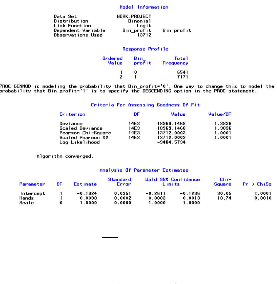
although probably still significant. The SAS output is seen in Figure 40.
Page 48
Figure 40
The regression equation is
Remember the regression equation should be converted to make is interpretable.
Shown below.
The estimated odds of a winning session multiply by
= 1.00080032 for each 1
hand increase in the number of hands per session. This is incredibly close to 1, meaning it
does not affect the estimated odds of a successful session very much. Here is another case
of a statistically significant predictor that is not practically significant.
Next I fit a multiple logistic regression model. I started with the saturated model and
started removing insignificant variables, starting with the least significant, until everything was
significant. Figure 41 shows the final model.

Page 49
Figure 41
It seems we are not going to see a lot of practical significance. The odds ratios are all
very close to zero. It is interesting that we yielded less significant variables in logistic
regression than regular multiple regression. Below is a chart of each estimate in exponential
form.
Figure 42
Variable Exp^estimate
Minutes played .9977
PFR% 1.0093
Aggression factor 1.03
WTSD% .9853

Page 50
W$SD 1.0500
All of these odds estimates are very close to one. This indicates that none of the predictors
practically significantly increase or decrease the predicted odds of a successful winning
session, holding all other variables constant. The logistic regression portion of the analysis
proved not to be as fruitful as expected. I was going to run a cross validation test but my
computer could not handle that many calculations and I am very confident the cross
validation test would yield results right around 50%, showing the model is better than random
guessing.
Outlier Analysis
I wanted to do an outlier analysis that would look at the all the extremely good and
bad results Mike had encountered. I wanted to look at the most winning and losing sessions
Mike endured and try to figure out why they happened. I also wanted to look at which players
have taken the most money from Mike and which players Mike has profited the most from.
Below is a chart showing the players Mike has profited from the most and who has won the
most against Mike.
Figure 43
Figure 43 shows the top three most winning and losing players vs. Mike. The largest
winner, BrynKenney has taken nearly 35 thousand from Mike. This is a very substantial
amount of money considering Mike has played against over 54,000 players. On the other
hand, Mike is up about 24 thousand against killer_ooooo. This is also very substantial. If you
consider the fact that Mike’s total profit is about 260 thousand and one player has accounted
for almost 10 percent of total profit, it is quite remarkable. The first thing I wanted to look at
was if there was any difference between the 3 winning players and 3 losing players as a
whole. I looked at a series of 2 sample t tests to see if there were any differences in the style
of play between the 3 winning players and the three losing players. Each test was a two
sided test. It is very important to note that I only looked at these tests and their p-values
informally and only as a starting point. Since there was certainly no random sampling going
on here in the outlier analysis. Any procedures in Figure 44 are informal.
Figure 44
Two
-
sample T for
Minutes Played
win lost N
Mean StDev SE Mean

Page 51
mike lost 173 36.4 46.2 3.5
mike won 461 38.1 35.2 1.6
Difference = mu (mike lost)
-
mu (mike won)
Estimate for difference:
-
1.66
95% CI for difference: (
-
9.30, 5.98)
T
-
Test of difference = 0 (vs not =):
T
-
Value =
-
0.43 P
-
Value = 0.669 DF = 250
Two
-
sample T for
Hands
win lost N Mean StDev SE Mean
mike lost 173 56.3 72.8 5.5
mike won 461 53.6 49.2 2.3
Difference = mu (mike lost)
-
mu (mike won)
Estimate for difference:
2.68
95% CI for difference: (
-
9.13, 14.48)
T
-
Test of difference = 0 (vs not =): T
-
Value = 0.45 P
-
Value = 0.656 DF = 233
Two
-
sample T for
Avg Players
win lost N Mean StDev SE Mean
mike lost 173 5.88 1.27 0.096
mike won 461
5.561 0.708 0.033
Difference = mu (mike lost)
-
mu (mike won)
Estimate for difference: 0.318
95% CI for difference: (0.118, 0.519)
T
-
Test of difference = 0 (vs not =): T
-
Value = 3.13
P
-
Value = 0.002
DF = 213
Two
-
sample T for
VPIP%
win
lost N Mean StDev SE Mean
mike lost 173 29.0 16.3 1.2
mike won 460 23.9 12.8 0.60
Difference = mu (mike lost)
-
mu (mike won)
Estimate for difference: 5.10
95% CI for difference: (2.39, 7.82)
T
-
Test of difference = 0 (vs not =): T
-
Value = 3.71
P
-
Value = 0.000
DF = 255
Two
-
sample T for
PFR%
win lost N Mean StDev SE Mean
mike lost 173 21.0 15.7 1.2
mike won 460 17.6 10.6 0.49
Difference = mu (mike lost)
-
mu
(mike won)
Estimate for difference: 3.40
95% CI for difference: (0.86, 5.95)
T
-
Test of difference = 0 (vs not =): T
-
Value = 2.63
P
-
Value = 0.009
DF = 233
Two
-
sample T for
3Bet%
win lost N Mean StDev SE Mean
mike lost 173 6.9 10.9
0.83
mike won 461 6.57 9.00 0.42
Difference = mu (mike lost)
-
mu (mike won)
Estimate for difference: 0.326
95% CI for difference: (
-
1.503, 2.156)
T
-
Test of difference = 0 (vs not =): T
-
Value = 0.35 P
-
Value = 0.726 DF = 264
Two
-
sample T for
Agg Factor
win lost N Mean StDev SE Mean
mike lost 173 2.61 2.72 0.21
mike won 461 3.59 4.21 0.20
Difference = mu (mike lost)
-
mu (mike won)
Estimate for difference:
-
0.977
95% CI for difference:
(
-
1.537,
-
0.417)
T
-
Test of difference = 0 (vs not =): T
-
Value =
-
3.43
P
-
Value = 0.001
DF = 475
Two
-
sample T for
WTSD%
win lost N Mean StDev SE Mean

Page 52
mike lost 173 21.5 21.4 1.6
mike won 461 21.1 23.5 1.1
Difference =
mu (mike lost)
-
mu (mike won)
Estimate for difference: 0.40
95% CI for difference: (
-
3.46, 4.26)
T
-
Test of difference = 0 (vs not =): T
-
Value = 0.20 P
-
Value = 0.838 DF = 337
Two
-
sample T for
W$SD%
win lost N Mean StDev SE Mean
mike
lost 173 38.9 39.3 3.0
mike won 461 33.3 39.7 1.8
Difference = mu (mike lost)
-
mu (mike won)
Estimate for difference: 5.63
95% CI for difference: (
-
1.28, 12.55)
T
-
Test of difference = 0 (vs not =): T
-
Value = 1.60 P
-
Value = 0.110
DF = 311
Again, it is important to note that these P-values are not valid because these are not random
samples. I simply used them as a guide to measure some differences.
Average players, VPIP%, PFR%, and agg factor yielded significant P-values at the
alpha = .01 level. I am not so sure that there is a practical difference between the two groups
in terms of average players. Both groups seem to be playing in 6 max games. There does
seem to be a practical difference for VPIP%. The players that beat Mike had a much higher
VPIP% than those who lost money to Mike. This means that players that are more willing to
put money in the pot did better against Mike. This makes sense because a lot of Mike’s
game is trying to get other people to fold their hands. PFR% was also significantly different
for the two groups. It was higher for the players that took money from Mike. This also makes
sense in terms of Mike’s strategy because his aggressive style works better against people
who do not raise pre flop because Mike wants to be the only pre flop raiser. Aggression
factor was also significant. Less aggressive players can take advantage of Mike’s aggressive
play. In this case Mike did better against players that had a higher aggression factor. It might
be the case that since Mike plays aggressively he can take advantage of other players that
play aggressive as long as Mike is more aggressive. Mike’s own aggression factor is 4.45,
which is higher than both groups which may account for this.
Now I wanted to look at Mike’s best and worst sessions. I was not sure whether to
qualify the best and worst in terms of straight profit or bb/100. Below in Figure 45 is a scatter
plot of bb/100 vs profit.

Page 53
Figure 45
I circled the sessions that I deemed outliers that I wanted to do additional analysis on.
Figure 45 looks interesting because there is no data in quadrants II and IV. This
makes sense because you cannot have a positive win rate and negative profit and vice
versa. The plot is fairly symmetric however if examined carefully you can see that there are
more very negative profit sessions and they are a lot more negative than the most positive
sessions. We have seen this before in this report. Mike wins more often than he loses but
when he loses he tends to lose a lot more money.
Figure 46 is the same chart shown earlier (Figure 10) but is included again to reference and
compare Mike’s normal play to the outlier sessions.

Page 54
Figure 46
Game Type Hands $ bb/100 VPIP% PFR% 3Bet% WTSD% W$SD% Agg Agg%
$25/50 NL 13949 ($57,361.20) -8.22 34.7 25 7.7 26.4 45.5 2.89 40.3
$30/60 LIM 205 $354.00
5.76 34 26.6 14.9 54.8 50 1.96 55
$10/20 NL 26601 ($22,627.95) -4.25 32.9 23.4 6.8 25.5 46.3 3 39.2
$15/30 LIM 56 ($634.00) -75.48 30.4 19.6 12 52.9 22.2 2.18 61.1
$5/10 NL 420238 $109,459.35
2.6 29.7 21 6.1 26.2 48.3 3 38.7
$10/20 LIM 371 ($1,436.50) -38.72 45.5 34.4 21.5 53 36.4 2.15 57.5
$3/6 NL 14360 $6,692.25
7.77 34 22.5 5.3 26.8 44.7 2.77 38
$5/10 LIM 2768 $999.00
7.22 40 25.8 11.9 37.1 48.9 2.57 52
$2/4 NL 1226761 $229,560.75
4.68 29.8 20.6 5.3 25.6 47.3 3.12 38.8
$4/8 LIM 4 ($50.00) -312.5 25 0 0 100 0 na 100
$2/4 LIM 105 $44.50
21.19 51 37 27.6 41.9 38.9 2.29 60
$1/2 NL 88156 ($6,348.75) -3.6 32.3 24.1 8.3 26.2 45.1 3.16 42
$1/2 LIM 10 ($21.60) -216 60 20 0 33.3 50 1.25 38.5
$0.5/1 NL 6446 ($424.55) -6.59 42.6 24.8 4.4 25.6 42.4 3.14 37.7
$0.25/0.5
NL 82409 $3,952.95
9.59 34 21.5 4.8 26.7 47 3 36.5
$0.5/1 LIM 23 ($13.25) -115.2 68.2 31.8 0 20 0 2.5 48.4
$0.1/0.25
NL 878 $14.60
6.65 32 23.4 6.7 19 40.5 4.44 54.5
$0.05/0.1
NL 318
($12.85) -40.41 26.8 22.2 3.3 30.4 38.1 4.14 41.7
$0.02/0.05
NL 96 ($10.21) -212.7 43.8 22.9 30.8 19.1 11.1 3.18 41.7
$0.02/0.04
LIM 19
($0.31) -81.58 84.2 57.9 0 42.1 37.5 1.45 65.1
$0.01/0.02
NL 159 ($14.28) -449.1 87.7 77.9 40.6 85.4 42.1 4.2 8.4
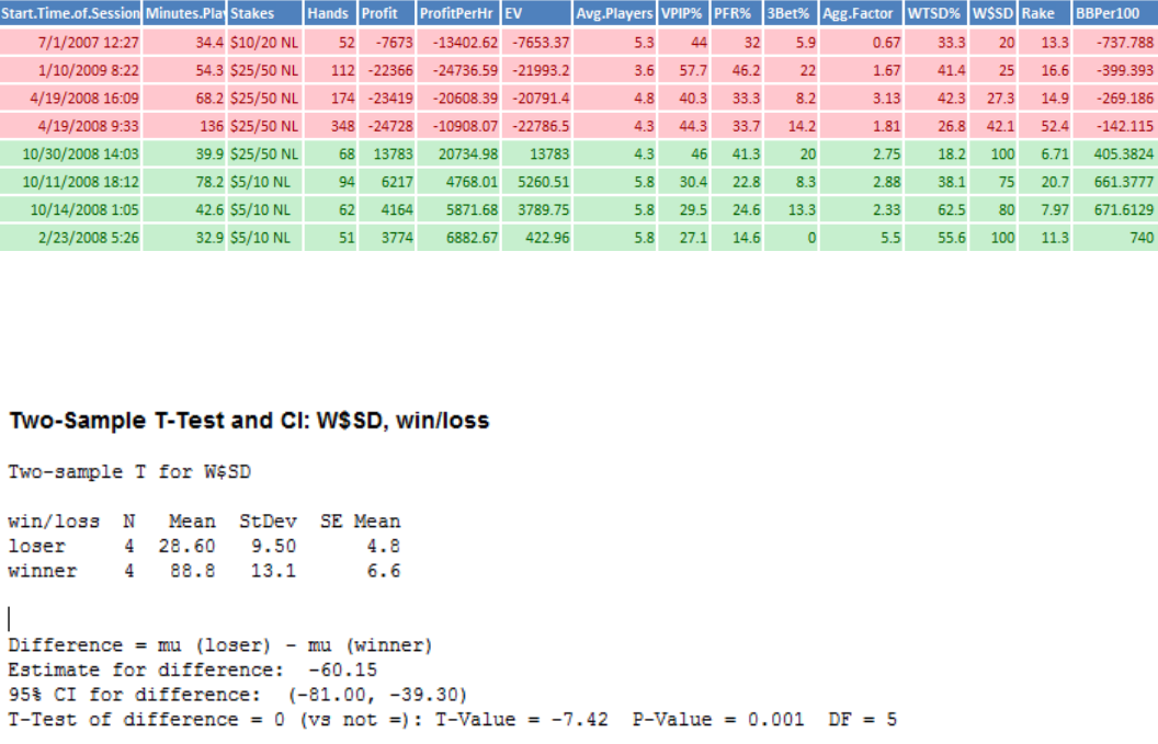
Below in Figure 47 shows the 8 outliers that I chose to analyze. You can compare Figure 46
to Figure 47 to see if Mike was playing any differently in his outlier sessions.
Page 55
Figure 47
You can already tell there are some differences in the winning and losing outlier sessions.
Figure 48
I performed t tests on each of the variables for the outlier sessions. There was only one
significant test, shown in Figure 48. Again, these are not valid t-tests but only there to get a
gage of what the differences are.
In the winning outlier sessions Mike’s W$SD percentage was higher than the losing
sessions. This variable seems to be coming up a lot in analysis as a key component. The
only way to win money without it coming on the river is to have everyone else in the hand fold
to your bet. Often times the biggest bets are made on the river. If a player is able to have the
best hand at showdown then he is guaranteed the biggest pot possible. To a certain extent
having the best hand at showdown comes down to what you were dealt which is based on
luck. The skill is knowing when to make it to showdown with your cards. In these outlier
sessions Mike was able to hold the best cards at showdown a very high percentage of the
time. Holding the best cards at showdown contributes to a very lucrative session.
The rest of the variables were not statistically significant however, since the sample
size for each group is only four and they are not random samples it might be more effective
to just examine the differences in the variables informally. Besides the one losing session at
10/20 the losing sessions are a lot longer than the winning sessions. This reinforces my
original hypothesis that the longer he plays the worse he does. After he has made a lot of

Page 56
money he might be more inclined to quit because he is satisfied with his winnings. If he has
lost a lot of money he might be more inclined to play more because he thinks he can win it all
back. VPIP% is also higher in almost every winning session. A higher VPIP% indicates a
looser playing style which is more inclined to spew money to opponents. Mike’s aggression
factor was also quite a bit higher in most of his winning sessions. Conventional wisdom says
that being aggressive is almost always better than being passive. At Mike’s most winning
stake his aggression factor was about 4.5 which is certainly higher than all the losing
sessions.
I was curious to see what the regression model would predict for these outlier sessions. I
decided to enter the winning and losing sessions into the optimal regression equations I
found earlier and find point estimates and confidence intervals. Seen in Figure 48 and 49.
Figure 48
Losing outlier sessions.
Compared to the actual -387 average win rate that Mike achieved over these 4 worst
sessions, the predicted fit of -42.8 is not actually that low. The size of the residual is very
large; however, it does show that the model did predict him to lose money.

Page 57
Figure 49
Winning outlier sessions.
The actual average win rate for these 4 most wining sessions was 619.6. This is a lot
higher than the estimate or the confidence limits. This might indicate that luck may have
been an important factor in these sessions.
The winning and losing outlier sessions were not identical. This is to say that it was
not just really bad luck or good luck to account for the differences. Perhaps if Mike had used
a different playing style he could have turned the monstrously bad sessions into moderately
bad sessions. After all, if Mike had decided to go play basketball instead of play in these four
bad sessions he would be up another 78,000 dollars or 30% of total profit. (Just something
to think about).
Conclusions
Suggestions for Mike
The whole purpose for this report was to figure a way to make Mike more profitable.
My thought was that I could use my skills in statistics to do a thorough report and figure out a
method to increase profit. One such hope I had was that I could tell Mike at what point in his
session that he should quit. An optimal playing time was not found. My results slightly
suggest that the longer the session, the worse it goes. I think the better advice is to continue
a session when you are playing well and end a session when you are not. My other goal was
to define what is playing well and what is playing poorly. I was not able to fully accomplish
this goal either. I think poker is too dependent on what the other players are doing at the
table to only look at one player’s stats. However, I did find that Mike wins more table
sessions than he loses (717 more). However, his biggest losing sessions are a lot bigger
than his biggest wining sessions. Cēterīs paribus, the higher the stakes the better the
players and higher potential for great loss. The most money in terms of profit and win rate
was no limit 400. My advice would be to continue at that level. Every once in a while I think it
would be profitable to look at your recent stats and make sure you are staying in line with
your winning strategy. Even though I was not able to find an overwhelming amount of
Page 58
evidence to suggest the explanatory variables explain everything, I was able to find to some
evidence they are important.
Overview
This project was plagued with one big problem. There was way too much data.
Throughout the entire report I had issues with finding statistical significance but not practical
significance. At the beginning of the project I was very optimistic to find some significant
results. It was disappointing that I was not able to find something more concrete. I had
always thought that there was always an optimal move in poker. I thought eventually some
super computer would be built that could beat the game of poker, similar to chess, well
almost beat. After this report I think that the game is too dependent on what the other players
at the table are doing. So often I hear Mike say something along the lines of, “oh, this guy
always check raises the turn”, or something to that extent. The problem with my analysis
was that it solely dependent on what Mike was doing. The model could not really take into
what other players were doing. I thought that since I was looking at averages I would take
into account all the different scenarios Mike could encounter. This did not seem to be the
case. I do think there is some value in looking at all the statistics. At the time of this report
Mike rarely, if ever, looks at personal or opponents stats. He thinks they over simplify things
too much. I am not sure if there is a way to optimize explanatory variables to maximize profit.
I also think that different playing styles will yield optimal results. However, I think for individual
players it is important to keep an eye on personal statistics. For instance if a player is in a
down swing he might want to make sure they are not changing their playing style from their
winning strategy. In short, I think my report was not able to show exactly the perfect way to
play, but showed that there is some value in looking at these variables.
What I learned?
I learned the pitfalls of having too much data. The power of each test I was making
simply way too much. I also learned the importance of having good notes. I was able to
reteach myself stat 418 in less than an hour. I hadn’t taken Stat 418 in over a year but I had
really good notes from Dr. Doi’s class and I am grateful I made them so nice to follow and
thorough. I also had to relearn a bit of SAS which I had not used in a while since switching to
R. Good notes were also helpful there. Stat 465 certainly helped me prepare for this report
but this definitely they largest report I have put together. I learned how to manage different
sections and put it together in a coherent manner. Lastly, Dr. Smidt did not set many, if any,
deadlines for me and I think I did a pretty good job at time management. I was able to make
sure everything got done in timely fashion.
