Is It Harder for Older Workers to Find Jobs? New and Improved Evidence from a Field Experiment

NBER WORKING PAPER SERIES

IS IT HARDER FOR OLDER WORKERS TO FIND JOBS? NEW AND IMPROVED

EVIDENCE FROM A FIELD EXPERIMENT

David Neumark

Ian Burn

Patrick Button

Working Paper 21669

http://www.nber.org/papers/w21669

NATIONAL BUREAU OF ECONOMIC RESEARCH

1050 Massachusetts Avenue

Cambridge, MA 02138

October 2015

We received generous support from the Alfred P. Sloan Foundation, and helpful comments from seminar

participants at Georgia State University, IZA, Marquette University, the New School, the Sloan Foundation,

UCI, the University of San Francisco, Stanford University, the University of Tokyo, the University

of Wisconsin, and Yale Law School. The views expressed are our own, and not those of the Foundation.

We thank Melody Dehghan, Dominique Dubria, Chenxu Guo, Stephanie Harrington, Kelsey Heider,

Matthew Jie, Irene Labadlabad, Benson Lao, Karl Jonas Lundstedt, Catherine Liu, Jason Ralston, Eileen

Raney, Nida Ratawessnant, Samantha Spallone, Bua Vanitsthian, Helen Yu, and especially Nanneh

Chehras for outstanding research assistance, and Scott Adams, Marc Bendick, Richard Johnson, Joanna

Lahey, and Matthew Notowidigdo for very helpful comments. This study was approved by UC Irvine’s

Institutional Review Board (HS#2013-9942). The views expressed herein are those of the authors

and do not necessarily reflect the views of the National Bureau of Economic Research.

At least one co-author has disclosed a financial relationship of potential relevance for this research.

Further information is available online at http://www.nber.org/papers/w21669.ack

NBER working papers are circulated for discussion and comment purposes. They have not been peer-

reviewed or been subject to the review by the NBER Board of Directors that accompanies official

NBER publications.

not to exceed two paragraphs, may be quoted without explicit permission provided that full credit,

including © notice, is given to the source.

Is It Harder for Older Workers to Find Jobs? New and Improved Evidence from a Field Experiment

David Neumark, Ian Burn, and Patrick Button

NBER Working Paper No. 21669

October 2015, Revised December 2015

JEL No. J14,J26,J7,K31

ABSTRACT

We design and implement a large-scale field experiment – a resume correspondence study – to address

a number of potential limitations of existing field experiments testing for age discrimination, which

may bias their results. One limitation that may bias these studies towards finding discrimination is

the practice of giving older and younger applicants similar experience in the job to which they are

applying, to make them "otherwise comparable." The second limitation arises because greater unobserved

differences in human capital investment of older applicants may bias existing field experiments against

finding age discrimination. We also study ages closer to retirement than in past studies, and use a

richer set of job profiles for older workers to test for differences associated with transitions to less

demanding jobs ("bridge jobs") at older ages. Based on evidence from over 40,000 job applications,

we find robust evidence of age discrimination in hiring against older women. But we find that there

is considerably less evidence of age discrimination against men after correcting for the potential biases

this study addresses.

David Neumark

Department of Economics

University of California at Irvine

3151 Social Science Plaza

Irvine, CA 92697

and NBER

[email protected]

Ian Burn

Department of Economics

University of California at Irvine

3151 Social Science Plaza

Irvine, CA 92697

[email protected]

Patrick Button

Department of Economics

Tulane University

6823 St. Charles Avenue

206 Tilton Hall

New Orleans, LA 70118

[email protected]

1. Introduction

Population aging in the United States and many advanced economies, coupled with the very low

employment rate of seniors, implies slowing labor force growth relative to population, and a rising

dependency ratio. This creates a public policy imperative to increase the employment of older individuals,

typically pursued via reforms to public pension systems (e.g., Gruber and Wise, 2007). In addition,

increased health and life expectancy implies a growing share of older individuals who plan to work longer,

even if these plans are not always realized (e.g., van Solinge and Henken, 2010). Efforts to extend work

lives – whether via public policy reforms to induce increased labor supply, or individual efforts to keep

working at older ages – may be thwarted by age discrimination in labor markets. This study utilizes a large-

scale field experiment to study whether age discrimination in hiring presents a significant barrier to

extending the work lives of older individuals.

Age discrimination in hiring is especially important in thinking about lengthening work lives, for

two reasons. First, a significant share of any increase in employment among seniors would be expected to

come from new employment in part-time or shorter-term “partial retirement” or “bridge jobs,” rather than

continued employment of workers in their long-term career jobs (Cahill et al., 2006; Johnson et al., 2009).

This path to retirement is likely driven in part by emerging health issues and other challenges as people age

(Johnson, 2014).

Of workers age 50 who report leaving their employer by age 70, 23% cite poor health as a

eason, and 58% report retirement as a reason (Johnson, 2014, Table 1). Perhaps reflecting these health

reasons, 36% of those age 50 who leave their employer by age 70 report changing occupations, although a

higher percentage (50) report moving to a different employer, suggesting that changing jobs but staying in

the same occupation can help older workers realize their goals. And workers who change employers for

reasons related to poor health report less physically demanding and less stressful work on their new jobs, as

well as fewer hours and more flexible schedules (Johnson, 2014, Table 4). Age discrimination in hiring

could interfere with these kinds of transitions to new jobs that let older workers extend their work lives. In

contrast, it seems likely that only modest changes in employment of older individuals are possible if

And workers may return to work after a period of retirement (e.g., Maestas, 2010).

difficulties in getting hired into new jobs limit older workers to staying in their long-term jobs a little longer.

Studying age discrimination in hiring is also potentially important because current policies to combat

age discrimination may be ineffective at reducing or eliminating age discrimination in hiring. Although

federal and state age discrimination laws have increased employment of protected workers, this effect has

likely come through reduced terminations (Neumark and Stock, 1999; Adams, 2004). These laws are likely

less effective at reducing discrimination in hiring because they rely on the legal process and hence on

potential rewards to plaintiffs’ attorneys. In hiring cases, it is difficult to identify a class of affected workers,

inhibiting class action suits and thus substantially limiting awards. In addition, economic damages can be

small in hiring cases because one employer’s action may extend a worker’s spell of unemployment only

modestly. (Terminations, in contrast, can entail substantial lost earnings, health insurance benefits, and

pension accruals.) And it could be worse: If age discrimination laws fail to reduce discrimination in hiring,

but make it harder to terminate older workers, these laws could actually deter hiring of older workers (Bloch,

1994; Lahey, 2008a; Posner, 1995). Evidence on the effects of age discrimination laws on hiring is scant and

somewhat mixed (Neumark and Button, 2014).

Existing field experiments generally – and nearly uniformly – point to substantial age discrimination

in hiring (Bendick et al., 1997; Bendick et al., 1999; Riach and Rich, 2006, 2010; Lahey, 2008b). But this

evidence is potentially flawed in ways that could bias estimates of age discrimination in existing studies

towards either overstating or understating discrimination. Consequently, we designed and implemented a

large-scale field experiment – a resume correspondence study – to address these potential limitations and

sources of bias in existing field experiments testing for age discrimination, which may bias their results. One

limitation that may bias these studies towards finding discrimination is the practice of giving older and

younger applicants similar experience in the job to which they are applying, to make them “otherwise

comparable.” The second limitation arises because greater unobserved differences in human capital

investment of older applicants may bias existing field experiments against finding age discrimination. We

also study ages closer to retirement than in past studies, and use a richer set of job profiles for older workers

to test for differences associated with transitions to less demanding jobs (“bridge jobs”) at older ages.

Based on evidence from over 40,000 job applications, we find robust evidence of age discrimination

in hiring against older women. But we find that the evidence for men is less robust, and that evidence of age

discrimination against them may at least in part reflect the biases this study was designed to assess.

2. Past Research on Age Discrimination

Evidence on Age Discrimination using Observational Data

The research literature on age discrimination is less extensive than the research on discrimination by

race and sex. One reason may be that the prima facie case for age discrimination is much weaker. For

example, unlike the cases with blacks or women, older workers generally have higher earnings than do other

workers. The other reason, almost certainly, is that aging does entail changing capacities, making it harder to

interpret differences in outcomes in observational data as necessarily reflecting age discrimination.

onetheless, a number of types of evidence from observational data are at least consistent with the presence

of age discrimination.

In the period prior to the passage of the Age Discrimination in Employment Act (ADEA), explicit

age restrictions in hiring ads were documented. In five cities in states without anti-age discrimination

statutes, nearly 60% of employers imposed upper age limits (usually between ages 45 and 55) on new hires

(U.S. Department of Labor, 1965).

A persistent finding is that older workers have longer unemployment durations than many other age

groups.

These longer durations need not reflect discrimination, however, and instead could arise from

igher reservation wages of unemployed older workers, owing to a higher value of leisure, expectations of

higher wage offers based on their most recent wage, etc.

There is substantial evidence of negative stereotypes regarding older workers, in hypothetical

However, it is hard to conclude that productivity during working ages clearly declines. Some research points to

relatively steady skills as workers age (e.g., Meier and Kerr, 1976); some research points to substantial declines in some

specific skills and performance-related behaviors, but improvements in other work-related characteristics, such as

leadership (Posner, 1995). Jablonski et al. (1990), based on evidence of actual output or piece-rate pay in a narrow set

of occupations, emphasize that in some occupations there is little or no evidence of productivity decline, and, more

generally, that the variation within age groups swamps average variation across age groups. See also Warr (1993).

Plant-level production functions for U.S. manufacturing workers also do not indicate productivity declines for those

aged 55 and older (Hellerstein et al., 1999).

For recent evidence, see http://www.bls.gov/cps/cpsaat31.pdf (viewed July 27, 2014).

scenarios tying attitudes toward older workers to adverse labor market outcomes for them (Finkelstein et al.,

1995; Kite et al., 2005), although more recent evidence suggests these negative stereotypes may have

declined in importance (Gordon and Arvey, 2004). Researchers have also noted the common and widespread

acceptance of ageist characterizations of workers, reflecting many of these stereotypes (e.g., McCann and

Giles, 2002; Eglit, 2014).

The research on negative stereotypes about older workers is also significant because it may help to

explain the nature of “age discrimination.” In particular, these stereotypes are consistent with statistical

discrimination. Alternatively, there may be simply animus towards older workers – perhaps not because of

“dislike” of older workers, but because of negative attributes associated with them that lead to the same kind

of disutility that drives the Becker (1971) model of discrimination.

There is also evidence that older workers “self-report” age discrimination. Such self-reports are

potentially problematic, because they can reflect other adverse outcomes that survey respondents attribute to

age discrimination. Thus, research studying the effects of these self-reports includes controls for job

satisfaction and other measures of workers’ perceptions of the workplace environment and fairness, and uses

longitudinal data on workers whose self-report changes to control for individual heterogeneity in the

propensity to report discrimination. Such studies indicate that workers who report experiencing age

discrimination subsequently exhibit more separations, lower employment, slower wage growth, and reduced

expectation of working past 62 or 65 (Johnson and Neumark, 1997; Adams, 2002).

ll told, this evidence based on observational data is generally consistent with the age

discrimination. But it is hard to interpret it as providing decisive evidence.

Experimental Research on Age Discrimination in Hiring

In the discrimination literature generally, experimental audit or correspondence (AC) studies of

hiring are viewed as the most reliable means of inferring discrimination (Hellerstein and Neumark, 2006; Fix

and Struyk, 1993). Observational studies try to control for variables that might be associated with

In the Lazear (1979) model of long-term incentive contracts (LTIC’s), employers can have economic motivations to

avoid hiring older workers. Whether the differential treatment of workers based on age implied by this model

represents discrimination may be a semantic issue; however, it has been interpreted as such from a legal perspective

(Issacharoff and Harris, 1997), as well as in the economics literature (e.g., Gottschalk, 1982; Cornwell et al., 1991).

productivity differences between groups, with questionable success. In contrast, AC studies create an

artificial pool of job applicants, among which there are intended to be no average differences by group, so

that differences in outcomes likely reflect discrimination. Audit studies use applicants coached to act alike,

and capture the outcome of actual job offers, while correspondence studies create fake applicants (on paper,

or electronically) and capture the outcome of “callbacks” for job interviews.

AC studies do have their critics (Heckman and Siegelman, 1993; Heckman, 1998). Audit studies

have received particular criticism because of the potential for “experimenter effects,” whereby the testers

may affect the outcome of the experiment through their behavior, and because of the difficulty of controlling

for all productivity-related differences that employers may observe. Correspondence studies avoid these

criticisms. They also have the major advantage of being able to send out thousands of job applications,

especially using the internet as more recent studies do. In contrast, even large-scale, expensive audit studies

typically have sample sizes in the hundreds (Turner et al., 1991), because of the time costs involved in

interviewing for jobs.

The principal downside of correspondence studies is probably that the researcher

bserves a callback for an interview (or some other positive response), rather than a job offer; we care most

about job offers, although callbacks are a prerequisite.

There is, however, one key criticism that carries over

rom audit to correspondence studies, discussed in the next section.

AC methods have been applied to age discrimination; the main studies are Bendick et al. (1997,

1999), Lahey (2008b), and Riach and Rich (2006, 2010).

In general, applications of these methods to age

In addition, current Institutional Review Board standards might deem audit studies unacceptable, because of the large

time required of interviewers for what are ultimately false job applications. In contrast, researchers (including us) have

successfully argued that the time spent reviewing electronic job applications is minimal, and hence that the benefits

from the knowledge gained from these studies outweighs these concerns. One study – which is short on details – claims

that on average recruiters spend 6 seconds looking at individual resumes (The Ladders, n.d.).

Pager (2007) suggests we may find less evidence of discrimination in correspondence studies, because an employer

may interview applicants from both groups tested, and only exert a biased decision at the job offer stage. That is not

necessarily true, though, since employers may be sensitive to hiring in an apparently non-discriminatory fashion from

those they interview for jobs. A related potential problem with inferring hiring discrimination from callbacks is that

callback rates may vary for groups when average qualification levels in the population differ, even though the intended

hiring rate for equally-qualified applicants is the same, because employers know there will more competition for the

highly-qualified members of the less-qualified group (Bertrand and Mullainathan, 2004). However, while this scenario

may be likely in studies of race discrimination, where minorities are disadvantaged relative to the rest of the population,

it seems unlikely to be factor in studies of age discrimination, where neither young nor old applicants would be

“surprisingly” qualified (or unqualified).

See also Albert et al. (2011), although their study only covers ages 24, 28, and 38, and hence does not speak to

discrimination follow the paradigm used in studies of discrimination against other groups, such as blacks or

women. Specifically, applicants are made identical (up to random variation) in all respects except age.

There is an issue in applying this paradigm to age discrimination, because of age-related differences in

experience. This, also, is discussed in the next section.

These studies – summarized in Table 1 – almost uniformly find evidence of age discrimination in

hiring. For example, Bendick et al.’s correspondence study (1997) looks at 32 and 57 year-old applicants.

Among applications in which at least one of the two applicants received a positive response, in 43% of cases

only younger applicant received the positive response, versus 16.5% of cases in which the older applicant

was favored, for a statistically significant difference of 26.5%. This difference is often referred to as “net

discrimination,” and ignores tests where both applicants have the same outcome.

Similar results are

eported in the other studies covered in Table 1, although there are some differences in results reported, and,

in one case, in the conclusion.

Note that the Riach and Rich and Bendick et al. papers are based on quite

small numbers of applications, for correspondence studies.

Bendick et al. (1999) report results that capture more than just whether the callback was positive. In

particular, they report the percentages of cases in which one paired tester received a more favorable response

than the other paired tester with “favorable responses” defined to include: an interview, an opportunity to

demonstrate skills, a job offer, or a job offer with higher compensation. In general, this echoes other features

of his study that try to capture more of the richness of the hiring/recruiting process, which is of course more

discrimination against older workers, in contrast to the other studies in which older workers are in their 50s or 60s.

Similarly, in a recent study Baert et al. (2015) study 38, 44, and 50 year-olds; this paper also discusses a couple of other

age discrimination studies.

The analyses reported in this paper simply focus on differences in callback rates in the sample as a whole, as has

become standard.

Lahey (2008b) reports rounded estimates suggesting only a marginally significant result, but estimates provided by the

author indicate that the difference is significant at the five-percent level. She reports the percentage of applications

resulting in interviews, but not the percentage of tests with one or more positive responses (or equivalently, the

distribution of responses based on whether only the older or only the young applicant received a call-back). Because of

this, we can only calculate a range of net discrimination estimates. At one extreme, using Massachusetts as an example,

assume that the results were generated by cases with both older and younger applicants offered interviews, or only

younger applicants offered interviews. In that case, 5.3% of applications resulted in one or more positive responses,

with 0% of the tests with positive responses favoring older applicants, and 28.3% (1.5/5.3) favoring younger applicants,

for a 28.3% net discrimination estimate. At the other extreme, if there was no overlap of positive responses, then 9.1%

of applications (5.3+3.8) resulted in at least one positive response, and the net discrimination rate is 16.5% (1.5/9.1).

Similar calculations for Florida yield a range of 18.1 to 30.6%.

feasible in an audit study than a correspondence study. Measured this way, the percentage of tests with a

more favorable response for younger applicants (age 32) was 42.2% for age 32, versus 1% for older

applicants (age 57), for a statistically significant difference of 41.2%.

Finally, the only contrary evidence comes from one of three cases in Riach and Rich’s (2010)

correspondence study in England. Specifically, for female applicants for jobs as retail managers, there was

statistically significant net discrimination against younger applicants (age 27 versus age 47) of 29.6% for

retail manager jobs. Still the other two estimates in this paper provide statistically significant evidence of

discrimination against older workers.

There are, however, two potentially important problems with this evidence, which this paper seeks to

overcome. These problems, and the proposed solutions, are described in the next section.

3. Limitations of Experimental Evidence on Age Discrimination in Hiring

Experience of Older and Younger Applicants

One problem specific to using AC methods to study age discrimination is that the usual approach of

making applicants identical (up to random variation) on all characteristics aside from the one in question is

problematic. Clearly, a young applicant cannot have the experience of a long-employed older worker. The

only option, then, is to give older and younger applicants the same low level of experience (commensurate

with the young applicants’ ages). However, this can make the older applicants in these studies look less

qualified than the older applicants employers usually see, which could explain why older applicants in AC

studies almost uniformly receive fewer job offers or callbacks. In other words, holding experience fixed may

bias the evidence from AC studies of age and hiring towards evidence of age discrimination.

Researchers are aware of this problem. Bendick et al. (1997) had both older and younger applicants

report 10 years of similar experience on their resumes. However, “[t]o account for older applicants’

additional 25 years of living not covered by their 10 years of experience” (p. 31), they had the resumes for

older applicants indicate that they had been out of the labor force raising children (for the female executive

secretary applications), or working as a high school teacher (for the male or mixed applications).

However,

xperience in unrelated fields, or time out of the labor force, could negatively affect employers’ assessments

of older applicants, generating spurious evidence of discrimination.

Lahey (2008b) focuses on women, for whom time out of the labor force is less likely to be a negative

signal than for men. She included only a 10-year job history, citing conversations with three human

resources professionals who said 10-year histories were the “gold standard” for resumes, and would not

convey a negative signal for older applicants. In addition, Lahey studies entry-level jobs, for which she

suggests that “job-specific human capital should be less of a concern” (p. 34). Nonetheless, a lack of

experience could be viewed as a negative.

In contrast, Riach and Rich (2006, 2010), who criticize this approach as using unrealistic resumes for

older workers, give their applicants experience more commensurate with their age.

Interestingly, as noted

arlier, one of three cases in one of these studies (Riach and Rich, 2010) reports evidence that does not point

to discrimination against older workers, but rather the opposite. However, the results are based on quite

small numbers of observations. Hence, between the small samples and mixed results we would argue that we

do not have a firm understanding of how the evidence on age discrimination in hiring depends on how

researcher treat the experience of older applicants.

Finally, in a recent study, Baert et al. (2015) also look at this question, which they label the

“Difference in Post-Education Years” problem. Looking at 38, 44, and 50 year-olds, they give all applicants

a job in the field to which they are applying for the same number of years prior to the application and

immediately after graduating from school. But they otherwise construct three different resume types: one

with inactivity in the “extra” years of older applicants, one with work in a different field, and one with work

in the same field. Their evidence points to lower callback rates for older workers only in the first two cases

Bendick et al. (1999) are vague, noting that their applicants indicate that they have several years of experience in an

occupation related to the job to which they are applying, and that the additional years of experience an older applicant

had accumulated were “ascribed” to a field unrelated to the position being sought, “such as military service of public

school teaching” (p. 9).

However, their resumes include only cursory descriptions of experience. In the 2006 paper, the resumes simply say

at the person has worked as a server in restaurants since about age 20. In the 2010 paper, one resume lists three jobs

held since age 17, rising to Senior Waiter, and the second has a paragraph description of the career since leaving school,

again with rising responsibility.

of out-of-field employment or inactivity. This evidence is consistent with bias towards finding age

discrimination when older resumes do not show greater continuous experience in the field. However, the

narrow age range used in this study (38-50) calls into question whether its results should even be compared

to the age discrimination literature. In addition, the study is based on a small number of tests (192 for each

type of resume). Moreover, their evidence by age (ignoring the issue of the difference in post-education

years) points to lower callback rates for 44 versus 38 year-olds and 50 versus 44 year-olds, but not 50 versus

38 year-olds (reflecting, in part, very different callback rates for 44 year-olds depending on whether their

applications are paired with 38 or 50 year-olds). Thus, even the overarching age patterns in this study are

unusual relative to the literature – although the age range is small and the upper age limit not very old.

We provide what we regard as more thorough and compelling evidence on the question of how

experience relative to age – and whether it is commensurate with age – affects the outcomes of these studies.

We conduct a much larger study, and we embed in the same experiment evidence from defining older

applicants as having the same experience as younger applicants, and defining them as having experience

commensurate with their age. Finally, we cover a much larger age range, and extend to what we view as a

very policy-relevant upper age range – near traditional retirement ages.

The Role of Unobservables

Another problem plagues AC studies of discrimination along any dimension. AC studies create

applicants who are identical in terms of variables observable to employers, and in a well-designed study –

especially a correspondence study that avoids issues like experimenter effects – we can assume that the mean

qualifications and characteristics presented to employers are identical across the two groups.

But even in the best case scenario of a well-designed correspondence study where we can assume no

differences in the means of unobservables, Heckman (1998) and Heckman and Siegelman (1993) show that

differences in the variances of the unobservables render the effect of discrimination unidentified, suggesting

discrimination where there is none, and vice versa. This is not an obscure statistical argument; differences in

the distributions of unobservable variables are a central element of models of statistical discrimination

(Aigner and Cain, 1977). Moreover, although it has not been noted previously, this problem can be

particularly important in studying age discrimination. In the human capital model, earnings become more

dispersed as workers age (after the overtaking age), because workers invest differentially in human capital

and these differences accumulate as workers age (Mincer, 1974). Given that this variation is unlikely to be

conveyed on the resumes used in correspondence studies, it presumably generates a larger variance of

unobservables for older versus younger applicants.

What is the potential implication? As Heckman (1998) shows, this difference in the variance of

unobservables interacts with the level of quality chosen for the resumes in a correspondence study. For

example, suppose the study uses relatively low-quality applicants, to avoid over-qualified applicants who do

not get any offers or callbacks. Then employers will favor the high variance group, since given the low

observed qualifications, the high variance group has a higher probability of having sufficiently high

qualifications to meet the hiring standard. In this case, there is bias in the direction of favoring older workers

in hiring, even if the resumes present similar quality and characteristics by age. Of course, the reverse

implication holds if the study uses high-quality applicants, since then employers avoid the high variance

group. Without knowing the quality of applicants employers actually receive, we do not know which

situation actually holds, and hence we do not necessarily know the direction of bias. As one example,

though, Bertrand and Mullainathan (2004, p. 995) claim that they tried to avoid over-qualified applicants

who employers might not bother trying to hire.

If past age discrimination AC studies have used relatively lower-quality applicants, and the variance

of the unobservable is higher for older workers, then – in contrast to the bias introduced by the “experience-

commensurate-with-age” problem – these past age discrimination AC studies are biased against finding age

discrimination. In that case, correcting for both potential sources of bias could, in principle, move the

evidence in either direction. Moreover, correcting for only one of them (as in the studies that, for older

applicants, use experience that is more commensurate with age) can increase the bias by eliminating one of

two sources of bias that are in offsetting directions. The next section of the paper explains, in general terms,

the approaches we take in this paper to correct for both sources of bias, and the following section then delves

into the details of the experimental design.

4. Empirical Approaches to Eliminating Biases in Correspondence Studies of Age Discrimination

Using Experience Commensurate with Age

In arguing that using older applicants with the same experience as younger applicants can create a

bias towards finding discrimination against older workers, we are taking a stand on what parameter we are

trying to estimate. In our view, there are both policy and legal arguments that the right comparison – and

hence the relevant parameter – is the difference in outcomes between younger applicants and older applicants

who have experience commensurate with their age.

The simpler argument concerns the policy question, which in our view is whether older job

applicants who are in some sense “typical” face difficulties in getting hired because of their age. For

example, media and research reports exploring whether age discrimination explains the long unemployment

durations faced by older workers during the Great Recession do not consider hypothetical older job

applicants who have not worked much and hence have equal experience to younger applicants; rather, they

focus on actual older job applicants who do have much more experience.

Similarly, Riach and Rich (2002)

rgued that “It makes more sense to acknowledge the heterogeneity and control for the differences to be

normally expected between the age groups being tested. Any differential response by employers to such

realistic human capital circumstances is of far more relevance to policy makers, than the artificial situation

contrived by Bendick et al. (1999)” (p. F508). Moreover, as the evidence described later suggests, how very

inexperienced older job applicants fare is arguably of less interest as a matter of public policy because there

are relatively few older job applicants in this category.

Perhaps more important, our reading of age discrimination law and legal rulings suggests that

evidence of age discrimination garnered from correspondence (or audit) studies using experience

commensurate with age, rather than equal experience, is more consonant with legal standards for age

discrimination. The ADEA makes it unlawful for employers to “fail or refuse to hire or to discharge any

See, e.g., http://www.nytimes.com/2013/02/03/business/americans-closest-to-retirement-were-hardest-hit-by-

ecession.html?pagewanted=all&_r=0 (viewed March 5, 2013); http://economix.blogs.nytimes.com/2011/05/06/older-

workers-without-jobs-face-longest-time-out-of-work/ (viewed March 5, 2013);

http://www.nytimes.com/2009/04/13/us/13age.html?pagewanted=all (viewed March 5, 2013); Mulvey (2011); and

AARP Public Policy Institute (n.d.).

individual or otherwise discriminate against any individual with respect to his compensation, terms,

conditions, or privileges of employment, because of such individual’s age.”

There is no mention, not

surprisingly, of comparisons at different levels of experience.

To consider what this means with regard to evidence from AC studies of hiring discrimination, it is

useful to review how discrimination is established legally. The standards for establishing an age

discrimination claim in a hiring case are fairly well-established, and a critical part of the standard, in a hiring

case, is that the plaintiff was qualified for the job and the defendant did not hire the plaintiff, yet continued to

seek applicants with the plaintiff’s qualifications (McDonnell Douglas v. Green, 1973; 411 U.S. at 792-793,

1973; Player, 1982-1983). These standards help establish a prima facie case for discrimination. If it is met,

then the burden of proof shifts to the employer “to articulate some legitimate, nondiscriminatory reason for

the employer’s rejection” (411 U.S. at 802), otherwise known as a “reasonable factor other than age”

(RFOA).

If the defendant does this, then the plaintiff has the burden of presenting additional evidence that

here was an illegal motivation for the decision (411 U.S. at 803-805).

In light of these standards, establishing that a decision not to hire an older worker was “because of an

individual’s age,” and hence illegal, would be much clearer in comparing a younger applicant to an older

applicant with experience commensurate with their age, rather than to an older applicants with unusually low

experience, which introduces another factor that could be construed as an RFOA. Suppose three applicants

are denoted: Y

(young, low experience), O

(old, low experience), and O

(old, high experience, i.e.,

xperience commensurate with age). Suppose that O

and O

are both passed up in favor of hiring Y

, while

and O

meet the prima facie standard of being qualified for the job (and not hired). The defense has to

offer a non-discriminatory reason for not hiring one of the other of the older applicants. It is clearly easier to

argue that O

was less qualified for the job than Y

, appealing to the lack of work for a good part of O

’s

career.

We suspect that this is the intent of the law: that the ADEA meant to protect typical older workers

See http://www.eeoc.gov/laws/statutes/adea.cfm (viewed August 4, 2014).

See http://www1.eeoc.gov//laws/regulations/adea_rfoa_qa_final_rule.cfm?renderforprint=1 (viewed August 4, 2014).

This last step is typical in disparate treatment cases, but is not always necessary in disparate impact cases (411 U.S. at

805; Tinkham, 2010).

from age discrimination, and hence to use a standard that, in the hiring context, defines discrimination in

hiring as adverse treatment of older applicants who are otherwise similar to younger applicants but have

experience commensurate with their age.

One possible counter-argument (Tinkham, 2010) is that an older employee with experience

commensurate to their age who has reached the same professional level as a younger employee is less

qualified, because it took him or her longer to reach that level. Regardless, O

would almost surely still be

egarded as an inferior applicant and hence discrimination against O

would be easier to defend, unless

employers truly regarded them as entering the labor market at an older age and hence having risen as fast as

. Moreover, for the low-skill jobs we study (as is typical of AC studies), it is hard to imagine that the

speed-of-success consideration is important.

Based on this discussion, we explore differences in results comparing young applicants (Y

) to older

applicants with low experience (O

) – as in other key age discrimination studies – as well as to older

applicants with experience commensurate with their age (O

). If low-experience resumes send a negative

signal, we expect less evidence of discrimination in comparing outcomes between young applicants and older

applicants with commensurate experience. And we have argued that the latter comparison is more relevant

to assessing whether there is age discrimination in hiring – on both policy grounds and legal grounds.

Correcting for Biases from Differences in the Variance of Unobservables

Neumark (2012) develops a method to address the “Heckman critique” of AC studies. Here, we

present a cursory discussion, beginning with the analytical framework for studying data from a conventional

AC study, and then using it to outline the method. The discussion is based on applications from only two

groups – older and younger applicants; although much of the study considers a wider variety of applicant

types, our work on the Heckman critique focuses on this simple two-way classification of applicants.

Productivity is assumed to depend on two individual characteristics, P(X’) = P(X

). X

denotes

bserved productivity measures included on the resumes. S denotes a dummy variable for age, with S = 1

for older (“senior”) individuals and 0 for younger ones. The treatment of a worker by an employer, which

depends on P and possibly S (if there is discrimination), is denoted T(P(X’),S).

Discrimination is defined as

(1) T(P(X’)|S = 1) ≠ T(P(X’)|S = 0).

Assume that P(.,.) and T(P(.,.)) are additive, so

(2) P(X’) = β

’X

+ X

(

3) T(P(X’),S) = P + γ’S.

γ’ is an additional linear, additive term that is intended to reflect taste discrimination against older

workers, equivalent to undervaluation of productivity). Two testers with either S = 1 or S = 0 apply for jobs.

The productivity measures are held constant in the study at a level denoted X

. Expected productivity for

lder and younger individuals are denoted P

and P

; these are based on X

, with X

unobserved by firms.

The goal of the usual AC study design is to set P

= P

Given these observables, the T is observed for each tester, and each test yields an observation

(4) T(P

,1) − T(P

,0) = P

+ γ’ − P

If P

= P

, then averaging across tests yields an estimate of γ’, or we can estimate γ’ from a

regression of the outcome T on a constant and the age indicator S

(5) T(S) = α’ + γ’S

+ ε

enote by X

and X

the values of X

and X

for older and younger applicants, j = I, II, with X

, and denote by X

the level at which X

is “standardized” across applicants. Then

(6) P

= β

’X

+ E(X

)

(7) P

= β

’X

+ E(X

In this case, each individual test provides an observation equal to

(8) T(P

,1) − T(P

,0) = γ’ + E(X

) − E(X

Clearly the data identify γ’ only if E(X

) = E(X

). Thus, a key assumption in AC studies is that

productivity-related factors not controlled for in the test have equal means for the two groups of applicants.

As discussed earlier, this can be hard to guarantee in an audit study using actual applicants, especially

because of experimenter effects. Correspondence studies make the assumption that E(X

) = E(X

) more

tenable, by avoiding face-to-face interviews that might convey mean differences on uncontrolled variables

between the two groups of applicants. Of course it is still possible that E(X

) ≠ E(X

). For example,

expected job tenure might be shorter for older workers. However, acting on such a belief would clearly

constitute statistical discrimination, which is illegal.

Thus, the estimated parameter from equation (8) has

to be interpreted as the sum of taste and statistical discrimination.

To see why differences in the variance of unobservables matters, assume that a job offer or interview

is given if a worker’s perceived productivity exceeds a threshold c’. Defining the treatment T as a hire (T =

1) or not (T = 0), the hiring rules for older and younger applicants are

(9) T(P(X

)|S = 1) = 1 if β

’X

+ X

+ γ’ > c’

(9’) T(P(X

)|S = 0) = 1 if β

’X

+ X

> c’.

Assume the unobservables X

and X

are normally distributed, with zero means, and standard

deviations σ

and σ

. The hiring probabilities for older and younger applicants are

(10) Pr[T(P(X

)|S = 1) = 1] = Φ[( β

’X

+ γ’ – c’)/σ

]

(10’) Pr[T(P(X

) |S = 0) = 1] = Φ[( β

’X

− c’)/σ

where Φ denotes the standard normal distribution function.

As equations (10) and (10’) show, even if γ’ = 0, so there is no discrimination, these two expressions

need not be equal because σ

and σ

, the standard deviations of X

and X

, can be unequal. More

generally, without knowledge or some restriction on σ

and σ

, γ’ is unidentified, which is the basis for the

Heckman/Siegelman claim that AC studies can be uninformative about discrimination.

EEOC regulations state: “An employer may not base hiring decisions on stereotypes and assumptions about a person's

race, color, religion, sex (including pregnancy), national origin, age (40 or older), disability or genetic information.”

(See http://www1.eeoc.gov//laws/practices/index.cfm?renderforprint=1, viewed September 27, 2015.)

Some AC studies try to distinguish between these hypotheses, by adding information to resumes and testing whether

differences in callback or job offer rates between groups are diminished (see Charles and Guryan, 2013); these studies

suggest that evidence of diminished differences imply that employers must have been statistically discriminating with

respect to the additional information. But we do not know, ex ante, on what characteristics employers might be

statistically discriminating, in which case a null finding that adding information does not change offer or callback rates

is uninformative. Also, a reduction in the difference between offer or callback rates from adding information to the

resumes does not necessarily imply statistical discrimination. To take an extreme case, suppose we compare results

using resumes with no information (i.e., only the group identifier), and with other typical information (like job

histories), and suppose that the callback or offer rate difference between the groups diminishes. This does not imply

that, in the real world, members of the disadvantaged group suffer from statistical discrimination, because hiring on the

basis of resumes with no information does not actually occur. Rather, we would need to know what information is

typically not provided in the job application process, on the basis of which employers statistically discriminate, and

examine the effect of adding that information.

To make explicit the point about bias made earlier, if X

is standardized at a low level, then β

’X

’. In this case, a larger variance for older workers, σ

> σ

, implies that we can find Φ[(β

’X

+ γ’ –

c’)/σ

] > Φ[( β

’X

− c’)/σ

] even when γ’ = 0. That is, there is a bias towards spurious evidence of

discrimination in favor of older workers, implying that correcting for this source of bias can lead to stronger

evidence of discrimination against older workers.

As shown in Neumark (2012), with a particular type of data from a correspondence study,

conditional on an identifying assumption, γ’ can be identified. The intuition is that a higher variance for one

group implies a smaller effect of observed characteristics on the probability that applicants from that group

meet the hiring standard. Thus, information on how variation in observable qualifications is related to

employment outcomes can be informative about the relative variance of the unobservables, and this, in turn,

can identify the effect of discrimination. Based on this idea, the identification problem is solved by assuming

that there is variation in some applicant characteristics in the study that affect productivity and that have

equal effects across groups. The typical AC study does not include such characteristics because applicants

are designed to be homogeneous. But if the applicants are made heterogeneous, this method can be used.

Formally, equations (10) and (10’) imply an age difference in hiring of

(11) Φ[( β

’X

+ γ’

– c’)/σ

] − Φ[( β

’X

− c’)/σ

A standard probit identifies coefficients only relative to the standard deviation of the unobservable,

so we normalize the variance of the unobservable to one. In this case, impose the normalization for young

applicants (σ

= 1). The variance of the unobservable for older applicants is then replaced by its variance

relative to the variance for younger applicants, denoted σ

S/Y

. The normalization is equivalent to defining all

of the coefficients in equation (11) as their ratios relative to σ

, denoted by dropping the prime subscripts,

so that the equation becomes

(11’) Φ[(β

+ γ − c)/σ

S/Y

] − Φ[β

− c].

We cannot tell whether the intercepts of the two probits in equation (11’) – and hence the hiring

probabilities – differ because γ ≠ 0 or because σ

S/Y

≠ 1. But if there is variation in the level of qualifications

used as controls (X

), and these qualifications affect hiring outcomes, then we can identify β

/σ

S/Y

and β

equation (11’), and the ratio of these two estimates provides an estimate of σ

S/Y

, and identification of σ

S/Y

implies identification of γ. The critical assumption to identify σ

S/Y

and hence γ is that β

is equal for young

and old applicants. Otherwise, the ratio of the two coefficients of X

for young and old applicants does not

identify σ

S/Y

. One can simply assume this, but when there are data on multiple productivity-related

characteristics (and this can be built into the study design) this assumption can be tested as the

overidentifying restriction that the ratios of coefficients on any variable measuring qualifications of older and

younger applicants are equal (to the same inverse of the ratio of the standard deviations of the unobservable).

/σ

S/Y

and β

can be estimated using a heteroscedastic probit model (Williams, 2009). Similar to

equation (5), letting i denote applicants and j firms, there is a latent variable for perceived productivity

relative to the threshold, assumed to be generated by

(12) T(P

) = − c + β

+ γS

+ ε

As is standard, it is assumed that E(ε

) = 0. But the variance is assumed to follow

(13) Var(ε

) = [exp(µ + ωS

)]

This model can be estimated via maximum likelihood. The normalization µ = 0 can be imposed,

given that there is an arbitrary normalization of the scale of the variance of one group (in this case the young,

with S

= 0). Then the estimate of exp(ω)

is exactly the estimate of σ

S/Y

The assumption that β

is the same for young and old applicants identifies γ. Observations on young

applicants identify –c and β

, and observations on old applicants identify (–c + γ)/exp(ω) and β

/exp(ω). The

ratio of β

/{β

/exp(ω)} identifies exp(ω), which, from equation (13), is the ratio of the standard deviation of

the unobservable for old relative to young applicants, identified from the ratio of the effect of X

on old

applicants relative to young applicants. With the estimate of exp(ω), along with the estimate of c identified

from young applicants, the expression (–c + γ)/exp(ω) identified from old applicants identifies γ as well.

The key to being able to use this method is to design job applications with more than one level of

qualifications. And if there are multiple measures of these qualifications, then the overidentification test can

be used. Thus, in the experimental design described later, we explain how we generate applicants of

different skill levels for each job for which we apply.

5. The Experimental Design

The standard procedures for correspondence studies are well established. There are three key steps:

creation of data on artificial job applicants; collection of data on hiring-related outcomes; and statistical

analysis. The usual statistical analysis without quality variation in resumes is straightforward, and the

extension to consider the Heckman critique closely follows what was described in the previous section. The

creation and collection of data, which includes both the design of the resumes and applying for jobs, is of

course central to the credibility and quality of the results from the experiment. This section describes these

aspects of the experimental design in considerable detail.

Creating Resumes

The resumes are the central element in the research project, since they constitute the “observations”

in the data. Three goals drive the design of the resumes. The first is to make choices (about target ages, for

example), that enable us to answer the most interesting questions. The second is to make the resumes as

realistic as possible, so that our artificial job applicants have the best chance of mirroring actual applicants to

jobs, and hence the results are most likely to be reflective of the experiences of actual job applicants. We do

this by grounding resume design decisions in empirically observable information, to the greatest extent

possible. And the third is to generate valid comparisons of older and younger applicants by, again, using an

empirically grounded approach to mimic actual resumes of older and younger workers.

Ages

We create resumes for older applicants chosen from two different age ranges. One set is assigned

ages 64, 65, or 66. These are older ages than used in past studies (Table 1). From a public policy

perspective, however, we are interested in people in the age range in which they are eligible for Social

Security benefits, in part because it is in this age range that retirement really accelerates (in part because of

these benefits), and because reforms aimed at extending work lives naturally focus on those currently eligible

for benefits. There is, for example, no talk of lowering the Full Retirement Age (FRA) in the future, but

there is talk of raising it (Business Roundtable, 2013). To better touch base with the existing literature, and

to explore differences as workers age, we also use middle-aged job applicants (aged 49, 50, or 51). These

ages are also of interest because an inability to find a job at these ages because of age discrimination can be

costly since Social Security benefits (and Medicare, for those aged 65 and over) are not available. Finally,

our younger applicants are aged 29, 30, or 31, in line with past studies. These are ages at which workers are

relatively young, but should have begun to develop some stability in their careers and hence to have built up

a resume identifying them as plausible and desirable applicants for the jobs to which they apply.

Bridge resumes

We also create variants of our resumes for the middle-aged and older workers that differ with respect

to whether these older workers have made or are making a transition to a lower-skill “bridge” job. For the

middle-aged applicants, these bridge resumes always show workers rising to higher-level jobs in the same

occupation before their current job application. We make the same types of resumes for the older applicants

as well, but also add a second type of bridge job resume in which applicants had shifted to a bridge job

around 8-10 years earlier. We do not construct the latter resumes for the middle-aged applicants because

they are much less likely to have made such a transition in their early- to mid-40s. In all cases, the bridge

resumes are created only for the high-experience resumes – the only ones that can exhibit the rising level of

jobs throughout the career and the possible downward career shift.

We have to introduce additional notation for our resumes for middle-aged and older workers. For

middle-aged workers, the resumes are distinguished by both experience (L or H) and, for the high-experience

resumes whether or not it is a bridge resume, so we use the notation {M

, M

, and M

HNB

} for the three

iddle-aged resumes (with B and NB denoting bridge and non-bridge). The older resumes are denoted {O

, O

, and O

HNB

}; the E and L superscripts indicate whether the transition to the bridge job occurs early

(i.e., 8-10 years before the current application) or late (contemporaneously with the current application).

Occupations

Given the constraints imposed by a correspondence study, we targeted jobs for which there are many

job ads on the internet (we use a particular job-listing website) and jobs that are fairly low skill, so that

electronic responses to these ads, providing resumes, can realistically be expected to generate requests for job

interviews. Not surprisingly, we therefore end up with some jobs that overlap those used in other studies.

To some extent, we targeted jobs in which there were some low-tenure older workers (which is not much of a

constraint since low-skill jobs tend to have high turnover) as well as low-tenure younger workers. In doing

so we tried to balance two conflicting issues. On the one hand, we wanted the resumes to be realistic,

avoiding jobs for which it would be very unusual for an older worker to apply. On the other hand, very low

representation of low-tenure older workers could reflect age discrimination. With age, as opposed to other

demographic characteristics, our view was that the former issue was predominant.

To get information on “new hires,” we used data from the 2008 and 2012 Current Population Survey

(CPS) tenure supplements to identify workers with fewer than five years of tenure.

We computed,

eparately for men and women, the shares of new hires in the age ranges 28-32 and 62-70,

relative to all

new hires in each occupation. Tables 2 and 3 present, for the 100 largest occupations (by employment), the

proportion of the young and old age groups indicated as a share of all new hires in the occupation, for men

and women. We have highlighted in boldface the occupations we use for this study. Lower-tenure older

men are quite common for retail salespersons, cashiers, janitors and building cleaners, and security guards.

These occupations also have sizable, but somewhat smaller, shares of low-tenure younger men, implying that

it would not be odd for an employer looking to fill these jobs to receive applications from both older and

younger men. Also, these four occupations typically do not require a significant amount of skills, training, or

experience, and are likely also accessible for older workers as partial retirement or bridge jobs. As shown in

Table 3, for women we choose some occupations that overlap those for men (retail salespersons and

cashiers), and some that are different (secretaries and administrative assistants, office clerks, receptionists

and information clerks, and file clerks).

Employer job advertisements are not categorized the same way as the Census Bureau classifies

occupations, as employers often lump sets of these occupations together (like administrative assistant and

secretary). We grouped the highlighted occupations from Tables 2 and 3 into four larger groupings of jobs,

for which we used common resumes: retail sales (corresponding to retail salespersons and cashiers in the

These are the Current Population Survey Displaced Worker, Employee Tenure, and Occupational Mobility

Supplement Files (see http://www.nber.org/cps/cpsjan12.pdf, viewed August 18, 2014). We avoided using the 2009

and 2010 CPS tenure supplements because of the Great Recession. The supplements are not available for 2011 or 2013.

These ranges are somewhat larger than the age ranges for our resumes (29-31, 64-66), to increase the sample size.

Census occupational classification); administrative assistant (secretaries and administrative assistants,

receptionists and information clerks, office clerks (general), and file clerks); janitors; and security guards

(security guards and gaming surveillance officers). These groupings were based on three criteria: how

different jobs related to these occupations were in the resumes posted on the web that we studied; how

different they were when employers looked to hire, based on job ads; and how many job postings were there

for these occupations. While the separate occupations may require slightly different skills and experience,

the core requirements and skills within these jobs are the same, allowing one resume to be used to apply to a

larger number of occupations. This has the added benefit of allowing us to avoid having to parse job

advertisements that are typically not written to fit into a Census occupation code niche, but rather fit broader

jobs that entail similar skills. Since the representation of people in these jobs and occupations differs by sex,

we only use male applicants for security guard and janitor jobs, and only female applicants for administrative

assistant jobs. Sales jobs are commonly held by both sexes, so for these jobs we use both male and female

applicants.

Our choices of jobs often overlap with past AC studies of age discrimination. One advantage of

using similar jobs is that differences in results are more likely to be due to methods than to differences in the

jobs studied. Lahey’s (2008b) study of women focuses on female-dominated jobs (like cashiers, secretaries,

and home health care). Riach and Rich (2010) studied waiters/waitresses and retail jobs.

igure 1 reports histograms, for all occupations with non-empty cells, for the share of hiring in each

age group relative to hires in the occupation (by sex). The figures also show the value of this share for the

occupations we use. For men, all of the occupations we use are fairly central in the distribution, although

security guards tend to have more older hires, and janitors more younger hires. For women the shares are

also in the mid-range of the distribution, although our occupations exhibit relatively more hiring of older

women and less hiring of younger women, suggesting that it is possible our results for women could be

biased against finding evidence of age discrimination.

Finally, we note that these are fairly low wage jobs,

The Bendick et al. studies (1997, 1999) use a wider variety of jobs.

Yet, as described later, our strongest evidence point to age discrimination against older women.

paying about 15-20% less than the median wage across all occupations, with the exception of administrative

jobs, which pay a bit above the median; see Appendix Table A1.

Cities

Because we apply for jobs in specific cities using our job-listing site, we needed to narrow the set of

cities used. Some past studies for the United States used a very small number of cities. Lahey (2008b) uses

Boston, MA, and St. Petersburg, FL, while Bendick et al.’s (1999) audit study is based on applications to

jobs only in the Washington, DC area. Other studies use a much broader geographic scope. Our goal in

choosing cities was two-fold. First, we wanted to include a large number of cities to help ensure that results

were not driven by city-specific idiosyncrasies. Second, we were interested in obtaining potentially

interesting comparisons across cities, although because many steps of the study entail a good deal of work

for each city covered, the number of cities was limited to 12. In particular, we focused on cities with

different age demographics, and cities with different state age discrimination statutes, to see whether either of

these dimensions is associated with different relative outcomes for younger and older applicants.

he differences in age discrimination statutes are based on research reported in Neumark and Song

(2013), which also indicated that the two key features of these laws that appear most important for

employment and retirement are larger damages for age discrimination claims, and whether the laws apply to

smaller firms than those covered by the ADEA (which covers firms with 20 or more employees). Thus, we

chose cities spread across states with neither type of age discrimination law (so the ADEA prevails), and

with one type of law or the other. We also chose some cities with a fairly old population more reflective of

the age structure towards which the U.S. population is evolving, as well as contrasting cities with younger

populations, based on American Community Survey (ACS) data.

The cities selected are displayed Table 4. Down the rows, the table groups cities from higher to

lower percentages of the population aged 62 and over. As the first number reported in parentheses after each

city indicates, this percentage ranges considerably, from a low of 11.6% in Salt Lake City to a high of 34.7%

In contrast, the geographic breakdowns by Census region in Bendick et al. (1997) are likely too broad to be tied to

either of these, and there is no variation in laws across the cities in the Riach and Rich studies (nor are any contrasts

drawn based on demographics).

in Sarasota. The “older” and “much older” cities are distinctly above the national average of 16.3% of the

population aged 62 and over, and the “younger” cities are distinctly below. The table also breaks these cities

into whether the state law allows larger damages under its age discrimination law. Of course, we might not

learn much that is reliable from 12 cities (in 11 states).

Job histories

Creating realistic resumes required a good understanding of how applicants for the jobs we target

actually portray their experience. There are a number of general issues, such as what type of information is

conveyed, what kinds of skill differences can be used to generate higher- and lower-quality applicants, etc.

And there are specific questions about differences between younger and older applicants, including the issue

of experience that is one central concern of this study.

To obtain this information, we downloaded publicly available resumes on a popular national job-

hunting website. This website has massive numbers of resumes.

The website allows some tailoring of

resume searches. We were able to search in the specific cities listed in Table 4, and to search for resumes

looking for the jobs we chose to target. To select resumes of older applicants, we also selected those whose

high school or college graduation dates would likely imply that they were age 50 or older. (Resumes

typically do not list age, but rather graduation dates.) Finally, we selected resumes with more than five years

of work experience, to focus on resumes of older applicants who were not new labor market entrants.

hile this search may not yield a representative sample of the universe of resumes of older applicants in the

jobs and cities we target, it does yield a large number of resumes in these cities and for these jobs. We

downloaded resumes, and then input relevant resume information into a database, including work experience,

work-related skills, education, approximate age, gender, and information on the pattern of work experience

For example, on August 13, 2014, searching for our jobs/occupations in Los Angeles yielded 72,835 sales associate

resumes, 1,809 janitor resumes, 57,660 administrative assistant resumes, and 8,222 security guard resumes, and in New

York City yielded 150,043 sales associate resumes, 2,418 janitor resumes, 121,394 administrative assistant resumes,

and 22,275 security guard resumes. The oldest resumes in terms of date posted were from late 2011. The resumes we

studied to design our resumes dated from August 2012. We did not use commercial websites for which terms-of-use

agreements precluded using them for our study.

The website also permits a restriction to resumes with more than 10 years of experience, but for the smaller cities and

ccupations, the weaker restriction was useful to obtain more resumes.

reported on the resume.

he main objective from using the resume database was to assist in the construction of the resumes.

Our first step in this process was to pool job titles and descriptions from the actual resumes to create a set of

entries to draw from for the work history sections of our fictitious resumes. We made minor changes to job

descriptions before we used them in our fictitious resumes, such as changing phrasing, grammar, specific job

details (like the number of supervisees), or the order in which job responsibilities are listed. The same

process was used to create entries for the “skills” section of the high-skilled resumes – discussed below.

For the construction of the non-bridge resumes, we combined these job descriptions using the resume

characteristic randomizer program created by Lahey and Beasley (2009). The program randomized the

combination of job titles and descriptions, and job tenures. The program runs backward from the most

current job to the beginning of the potential job history (1970). We had to build in a probability of a job

ending, and experimented with the randomizer to choose a probability that appeared to create job histories

similar to the resumes we downloaded, in terms of number of jobs held and average tenure on a job; this

iterative process led us to choose a 15% annual probability that the program will end the current job and

move on to the next randomly assigned job.

We used the resume randomizer to produce a large number of job histories, and then selected a

smaller set that looked the most realistic based on the resumes found on the job-hunting website. In

particular, we dropped those that had very high levels of turnover, unusual sequences of jobs (such as

repeatedly switching between a manager and a cashier, etc.), or long strings of employment in other

occupations (e.g., spent 20 of the 40 years as a real estate agent). From this sample of acceptable histories,

we created three job histories for each type of job and city. All job histories contained information going

back to 1970, so to create the job histories of younger applicants, as well as older applicants reporting low

experience, the job histories were truncated at the appropriate year. This way the most recent parts of the job

histories (roughly 2000-2014) look very similar across any of our resumes distinguished by either age or

Prior to creating any data based on the resumes we strip out the personal identifiers to protect the confidentiality of

the job applicants who posted the resumes.

experience.

We modified our process to create bridge resumes. Using information from job histories on real

resumes, we tried to match the patterns that workers exhibited. Two patterns stood out: a defined profile of

responsibility; and longer job tenure on the higher-responsibility jobs. More specifically, these resumes

showed a progression of jobs from low-level to high-level jobs. After progressing to increasingly more high-

level positions that lasted longer, these individuals would peak at a high-responsibility job. In some of the

resumes, they would then make a clear and pronounced downshift towards low-level jobs, which likely

parallels what the literature refers to as bridge jobs (Cahill et al., 2006; Johnson et al., 2009). Workers would

remain in bridge jobs until retiring.

To approximate these job profiles over time, we used jobs from our bank of actual resumes. Jobs

were coded according to their level of responsibility. Entry level, low-skill jobs were coded at 1, while the

most high-skill, high-level jobs were coded as a 5. The coding of jobs can be seen in Appendix Table A2. In

retail sales, the lowest responsibility job is a cashier or sales associate. Individuals work their way through

various levels of store management before peaking as a store manager. In security, workers start out as

entry-level security guards. They will peak at directors of security; note that for security we do not really see

mid-level jobs and therefore the career profiles go from jobs coded 1-2 to jobs coded as 5. For

administrative assistants, workers start as a receptionist before working their way to a peak job as an office

manager. Janitor resumes did not exhibit the same pattern of peaking and bridging that was found in other

occupations, so we did not create bridge resumes for janitors.

To create a bridge resume, we arranged jobs so each job history exhibited the desired peaking

behavior. All jobs held by these workers were within the same occupation. Each new job was the same level

or higher. After peaking at the highest available job, workers would continue at jobs at that level until they

downshifted to a bridge job. There were two types of bridge resumes: either with this downshift occurring 8-

10 years prior (for older applicants only), or currently in progress with the bridge job being the job for which

the person is applying. These bridge jobs are the same jobs that are used in the creation of the non-bridge

resumes (O

HNB

and O

). Appendix Figures A1-A2 provides a visual representation of the “profiles” of these

codes for the different resumes we created. These figures show how the level of responsibility evolves

differently in the bridge and non-bridge resumes we use.

On the real resumes tenure in these high-responsibility jobs is longer than tenure on low-skill jobs.

To adjust for this we used a lower annual transition probability (7.5%) to generate longer job tenures, so that

on average these workers will stay at these jobs twice as long as they do at the low-skill jobs.

The tenure at

ach job was created using the randomizer code described earlier and then added to the resumes. After the

worker downshifted to a low-skill bridge job, they had the same transition probability as other workers in our

fictitious sample for every job subsequently held. This was done so bridge jobs appear identical to the jobs

on the other resumes. The result is that all O

resumes will have very similar job histories to the O

HNB

and

resumes for their last 8-10 years.

We added employer names and addresses manually to each job on our final job histories. We

ensured that the job title and description was realistic for the employer. In addition, we used employers that

were active at the time and in the region listed, relying mainly on the actual resumes, supplemented by

additional research on chains. In some cases, we added large public or private institutions known to be open

in a particular period as employers. Employer names were added randomly if they were valid for the job.

These steps complete the construction of job histories used in the resumes. The remaining steps,

described below, concern other information that we needed to add to complete the resumes. All other resume

information was added to the resumes using Visual Basic for Applications (VBA) programs that we created.

Creating our own code allowed us to randomly add and track several resume characteristics. These included

adding school names and addresses to the education information, skill information to create high-skilled

resumes, current employment status, and then the more specific information that completes the resumes,

including applicant name, year of high school graduation to convey information on age,

and residential

With a constant hazard, the distribution of tenure is exponential, with mean equal to the inverse of the hazard. We

also use this lower transition probability for the earlier, lower-responsibility jobs for the bridge resumes, to distinguish

those more likely to progress to a higher-responsibility job at the same employer.

To reduce the number of job histories, we do not change the job history based on these small variations in age within

ur three-year age ranges; we only change age via the high school graduation year. This should have no bearing on our

results for differences across the three broad age groups, which is our focus. Also, it likely to be undetected because

most resumes do not go quite all the way back to the likely school leaving age.

address, as well as phone numbers and email address so that employers can contact the applicants. Our VBA

programs also grouped our completed resumes into triplets for us, created application scripts, saved our

resumes with file names reflecting the names on the resumes, and organized all these files an intuitive folder

structure.

In addition to using the database of resumes to construct our resumes, we also wanted to use it to

characterize real resumes more systematically, including documenting the age distribution of those looking

for jobs, as well as features of resumes for older workers – with a particular focus on the amount of

experience listed and trajectory of jobs held for those now applying to the jobs we were targeting. To this

end, in addition to our resume construction efforts, we drew a systematic sample of resumes from the website

from which to assemble this information. We first searched for resumes with more than two years of work

experience, in the four occupations and 12 cities used in our study, and in three experience groups (3-5 years,

6-10 years, or 10+ years). In each group we extracted the greater of all resumes listed or 1,000 resumes, for a

total of 25,460 resumes.

We then wrote code to extract information from the resume text.

ge is calculated based on the listed high school graduation year. Information on high school

attendance is reported on 81% of the collected resumes, and of these, 68% include high school graduation

year, reducing the sample to 14,316 resumes (56% of the total). We also determined the sex of applicants

based on matching names to SSA data; our method assigns gender to 82% of individuals, reducing the

sample to 11,751 individuals.

We calculate experience based on job history information, as the number

of years worked. If there are multiple jobs held at the same time, experience is not double-counted.

Resumes may be posted in multiple occupation categories. Based on name, age, and work experience, only 6% of the

resumes with available age information repeat in the sample. Omitting these resumes does not change the descriptive

results provided below.

We use data from a 100% sample of Social Security card applications for U.S. births. In each year the Social Security

Administration (SSA) records the number of males and females born with a name and reports frequency counts of those

names by sex, as long as the name is at least two characters long with a frequency of at least five. We match using first

name to the SSA data in an individual’s birth year. If a name applies to both males and females, we assign the majority

gender as long as at least 90% of children born with that name have the same gender.

Computed experience from the resumes corresponded to the experience “bins” used on the website. Average

omputed experience was 5.4 for the 3-5 year group, 9.2 years for the 6-10 group, and 17.6 years for the 10+ group.

Moreover, 34%, 40%, and 26% of cases had computed experience in the corresponding range. We would not expect an

exact correspondence since the experience bins are selected by job posters rather than constructed from resumes, and

hence may reflect other factors (like including experience only in the specific job for which the person is seeking work).

One finding was that – consistent with the CPS tenure supplement data showing some

representation of low-tenure, older workers in the jobs we study – there are many older workers looking

for jobs in these occupations. Figure 2 displays the age distribution of resumes in each of the four jobs we

study, although note that because we were more likely to cut off the number of resumes extracted at 1,000

for lower experience cells, there is a bias towards older resumes in these histograms.

Nonetheless, the

resence of older resumes on the website suggests that older workers do use on-line resources to apply for

jobs. As additional evidence that job search methods do not differ sharply between older and younger job

searchers, we examined data from the monthly CPS files for 2014 on job search methods among the

unemployed. As reported in Appendix Table A3, the distributions of job-search methods are fairly

similar across these age groups.

A second clear finding is that a large share of resumes of older applicants list job experience that is

commensurate with their age, including jobs going all the way back to the 1970s and even the 1960s for

those who were old enough; there was, in particular, no indication that older job applicants limited reported

work experience to 10 years.

This is reflected in Figure 3, which plots average experience by age – overall

in the top panel, and by job in the bottom panel. Both panels indicate that, on average, reported experience

on the resumes rises approximately linearly with age. This information, in our view, further justifies our

interest in differential treatment between younger job applicants and older job applicants with experience

commensurate with their age.

esume quality/skills

To be able to implement the correction for differences in the variance of unobservable, we designate

half the resumes to be high skilled (or high quality), and half to be low skilled. We chose quality- or skill-

We do not know the universe of resumes on the website, so there was no way to adjust for this.

While resumes for older workers did not always feature a complete job history indicating near-continuous work, there

was no consistent way that older workers explained gaps when they existed.

We also examined the persistence of careers within the same occupations, using phrases that appear to cover the same

jobs. Administrative assistant includes administrative, receptionist, office manager, file manager, file clerk, or

secretary; retail sales includes cashier, store manager, or sales clerk; security includes security guard or officer; and

janitor includes janitor, cleaner, maintenance, dishwasher, housekeeper, or custodian. Because we likely cannot classify

all job titles as accurately within the four jobs covered in the study, we assume that we obtain lower-bound estimates of

persistence. For each type of job included in the study, between 29 and 32% of all jobs were in the same job as the

current job for which the person was seeking work.

related items to include based on the actual resumes. These items show up in three ways on the resumes.

First, high-skill resumes can include a post-secondary degree, while all low-skill resumes only list a high

school diploma. These degrees were most commonly B.A. for sales, administrative assistant, and security

guard applicants, and Associate of Arts for janitor applicants.

Second, high-skill resumes include a “skills” section that can include computer skills of some kind

(appropriate to the job), and fluency in Spanish as a second language, and other occupation-specific skills.

Thus, aside from Spanish fluency and education, for administrative/secretarial jobs, the higher skills include

typing 45, 50, or 55 words per minute, and facility with computer software (showing a randomly chosen mix

of Quickbooks, Microsoft Office, and inventory management software). For retail/cashier jobs, the higher

skills include Microsoft Office and programs used to monitor inventory (VendPOS, AmberPOS, and

Lightspeed), and the ability to learn new programs. For security jobs, applicants are described as licensed in

their state, and their resumes show CPR training. For janitor jobs, the high-skilled resumes indicate a

certificate in using particular machines and a certification in janitorial and cleaning sciences. In addition, the

skills section can include one of three volunteer activities (food bank, homeless shelter, or animal shelter).

We also phrase the skills descriptions to match what we observed in our sample of resumes.

n addition to education and skills, we also use slight variations in resume quality. All low-quality or

low-skill resumes include two typos (one missing space and one missing period, with one of these appearing

for the most recent job, which employers are most likely to read). Some high-skill resumes do not, so we can

think of “purging” these errors as adding a skill.

Finally, some high-skill resumes include a description of

“employee of the month” awards on the most recent job.

We do not assign all of the skill or quality dimensions to every high-skill resume, because we obtain

valuable information (and the overidentification test) from being able to estimate the coefficients on different

skills in the heteroscedastic probit model. Rather, from the vector of skill or quality characteristics

We used the same sample of resumes described earlier to provide some tabulations of skills on actual resumes, based

on our scraping of these resumes for descriptions of skills. These are reported in Appendix Table A4, which shows the

prevalence of the skills we use on all resumes in all of our occupations (e.g., Spanish), and also the greater prevalence of

particular skills for specific occupations (e.g., Microsoft Office for administrative and sales resumes, CPR and first aid

for security resumes, and cleaning and related skills and certification for janitor resumes).

Typos and grammatical errors were more common on actual resumes than spelling errors.

(education, skills, interests, typos, and employee awards) we randomly assign five of seven possible skill

indicators to each high-skill resume. We assign all applicants within each triplet as either high skilled or low

skilled, with 50% probability for each. In contrast, control variables (resume characteristics) that are not

supposed to affect hiring are randomized across resumes in audit and correspondence studies. We make

triplets uniformly high-skill or low-skill because skill and age define different treatment groups, and we do

not want random assignment of high-skill or low-skill resumes within a triplet to dominate the effect of age.

Separations, employment, and unemployment

Some resumes list months only for very recent jobs, and some list them going further back. We use

months in the job histories to better match the majority of the resumes, varying across resumes whether or

not months are shown for much earlier jobs.

To mimic the actual seasonal pattern of job changes for

different types of jobs, we randomly draw the separation month for each job, except the most recently held

job, from the distribution of job separation dates from the Job Openings and Labor Turnover Survey

(JOLTS). We use the general monthly distribution of separations for janitor and security resumes, the

distribution specific to “Retail Trade” for sales resumes, and the distribution specific to “Business Services”

for the administrative assistant resumes. During the course of the field experiment, every month we moved

the ending date of the most recent job forward one month, so that durations did not lengthen during the time

the experiment was in the field. We distinguish resumes based on whether applicants are currently

unemployed.

We assign all applicants within each triplet as either all employed (the most recent job end

ate listed as “Present”), or all unemployed, with 50% probability for each. When applicants are

unemployed, the resumes indicate that their last job ended in the month prior to the job application.

Applicant names and age

Applicant names were selected randomly from a set of the most common first names and last names

for the relevant cohorts. This information was taken from the Social Security Administration list of most

And when months are shown, job transitions vary randomly as to whether they occurred in the same month, one

month later, two months later, or three months later.

Kroft et al. (2013) use a correspondence study to estimate the effects of duration of unemployment on hiring of the

unemployed.

popular baby names.

We chose first and last names that were most likely to signal that the applicant was

aucasian, by excluding names where fewer than 60% of individuals with the name were Caucasian.

All

applicants, regardless of age or gender, had last names randomly assigned from the same selected set of last

names. For first names, we created six separate sets of first names to draw randomly from each age group

(64 to 66, 49 to 51, and 29 to 31) and sex, using the most common first names for those groups.

We chose

he 20 most common names for babies born in each corresponding birth year, dropping names that were

gender ambiguous unless using the full name made this clear (e.g., Patrick instead of Pat). The composition

of names for the middle and older categories were very similar so we combined these categories before

choosing our most common names for applicants in each age group.

Residential addresses

Addresses on the resumes were selected carefully to ensure that they were realistic for both older and

younger applicants, did not signal a race other than white, and were not likely to send an unusual signal

(positive or negative) about the applicant. We first chose zip codes that were not too far from the central

business district(s) in the metro areas (or the center of the sub-markets used on the job-posting website, as

explained in more detail below),

so that an employer would not be less likely to offer a job to those

erceived as having an excessive commute.

We also chose zip codes that were not sparsely populated, and

did not have high or low unemployment, family income, share black, or shares of old or young residents.

We began with all zip codes entirely contained within the Core Based Statistical Area (CBSA),

See http://www.ssa.gov/OACT/babynames/ (viewed August 11, 2014).

We use U.S. Census records on most common last names in the 2000 Census for last names. The 2010 data were not

available when we chose the names. However, there were only minor changes from 1990 to 2000, so we suspect that

using the 2000 list is not problematic. (See http://www.census.gov/genealogy/www/data/2000surnames/surnames.pdf

and http://www.census.gov/genealogy/www/data/1990surnames/index.html, both viewed August 11, 2014.)

We draw randomly from these age ranges, and then assign year of high school graduation to resumes, assuming

people graduated at age 18 and are currently older by the number of years between the year of high school graduation

and when job applications went out (2015). Since not everyone graduates at age 18, and since some who did graduate at

age 18 could have been a year younger than the bottom of each age range if their birthday was between the month and

day of high school graduation and the month and day the application went out, employers could have assumed slight

deviations from our intended age ranges.

Sub-markets are regions within a city’s market.

Data from the 2009 American Community Survey indicate that over 50% of (one-way) commute times to work are 24

inutes or less in length, and only fewer than 15% are 45 minutes or longer (U.S. Census Bureau, 2011).

Census-defined metropolitan areas that capture a labor market within which people commute.

We used

ata at the zip code level from the American Community Survey (ACS) to exclude any zip codes for which

the characteristics listed above were unusual. To avoid sparsely populated areas, we exclude zip codes in the

bottom quintile of the total population distribution across zip codes in the CBSA. We first exclude zip codes

in the bottom quintile of the proportion of the population aged 25 to 34, 60 to 64, or 65 to 74. We then also

exclude any zip codes that have an age distribution that suggests far younger residents than older residents,

or vice versa, based on the ratio of those aged 60 to 74 to those 25 to 34.

In addition, we drop zip codes in

he top or bottom quintiles of the distributions of the unemployment rate or median family income, or if the

share black is in the top quintile of the distribution (areas with a low share black are not problematic, as there

are many of them). We also exclude military bases and similar areas.

Among the zip codes that remain after imposing these restrictions, we drop zip codes that are more

than 25 miles from the central location of the corresponding job market for the job posting locations we use

to identify jobs. For central areas, we use the central business district, excluding zip codes more than 25

miles from the center of the zip code to city hall. For sub-markets on the job-posting website, we use

distance from the zip code to the center of the sub-market, using city hall if the sub-market included it, and

otherwise approximating by visual inspection of maps. Distances are measured using Google Maps,

assuming travel by car; Google maps calculates these based on geographic centers of zip codes, except for

downtown areas where it uses the city hall. Table 5 shows, as an example, the zip codes selected for the

New York City CBSA and the associated sub-markets. We present summary statistics for the entire CBSA,

and then for each zip code we selected. Appendix Table A5 shows all of the zip codes used.

We then assign street addresses for the zip code, using Zillow to select streets and addresses so that

house prices at the address are about average for the metro area (having already selected zip codes with

intermediate values of median family income). For each zip code selected, we search on Zillow for all

See http://www.census.gov/geo/reference/gtc/gtc_cbsa.html (viewed August 11, 2014).

We do not simply use percentiles of the distribution, because in some cities that have particularly old populations, the

atio of old to young residents can be quite high even at the bottom of the distribution, for example. We thus base our

exclusion rules for the ratio of young to old on a hybrid of relative and absolute criteria, dropping zip codes with the

ratio of older to younger residents below the minimum of 0.5 and the 20

percentile, and above the maximum of 2 and

the 80

percentile.

houses for sale or rent, and pick a street where prices were near the averages for the city. We then utilized

the “street view” function to select streets that were primarily residential, rather than a mix of residential and

business, and to determine if the majority of buildings on the street were apartment buildings or detached

houses. Once a suitable street was found, we picked a house to get the exact address (123 Main Street for

example) and then used that to create a range of numbers around the house to draw from for our addresses

based on 100s (so 100-200, in this example). For streets with mostly apartments, we assigned apartment

numbers, choosing randomly from two to nine.

Within each triplet of applications sent in response to an ad, all applications were from different zip

codes and different addresses. These were randomly assigned so that applicants with certain characteristics

do not have tendencies to be from different kinds of neighborhoods (or homes). Using zip codes and

addresses that are not outliers ensures that within triplets applicants are similar on these dimensions.

Phone numbers and email addresses

The resumes had to include information that employers could use to contact our fictitious applicants,

which is how we collect data on outcomes of the hiring process. We purchased “online” phone numbers for

our applicants using Vumber. These do not appear any different than regular phone numbers to the

employer, but have the benefit that the calls and voicemails are recorded in an online account and no physical

phones are required.

We selected phone number area codes for all applicants that were located centrally in each metro

area whenever possible. From the set of centrally-located area codes, we tried to avoid picking those that

were too old, as these may be difficult to get or are considered “posh” (e.g., 212 in Manhattan), or too young,

such that it might be far more likely that the area code would belong to someone younger (e.g., 929 in New

York, which was only created in 2010). Table 6 presents the area codes we used for each metro area, along

with information on their coverage areas and dates of creation. Four of the area codes we use were ones that

were the first to be assigned to the area, in 1947, in some cases because other area codes that covered a

similar geographic area were overlaid too recently. In Birmingham, there is only area code (205). In

We give credit for some of the ideas in this subsection to an earlier correspondence study by Figinski (2013).

Phoenix, there were not enough 602 area code numbers available from our provider that were unique enough

from each other, so we assigned each of the three applicants to a different area code in the greater Phoenix

area (602, 480, and 623).

When employers respond by phone, they may not always leave a message that provides enough

information to match them to an exact applicant (let alone job ad). Assigning a unique phone number to

every job applicant and job ad would solve this problem, but is prohibitively expensive and complicated.

e purchased enough phone numbers to assign unique numbers to each group of job applicants defined by

occupation (administrative assistant, janitor, sales, and security), city, sex (for sales, where applicants are

either male or female), and type of triplet that the resume is a part of (triplet with two resumes of age 64-66,

two resumes of age 49-51, or one of each, along with a young applicant). This results in 360 unique phone

numbers. With all of these numbers, it is very unlikely that we would not be able to assign a response to an

applicant, although assigning it to a unique job ad requires more information (discussed below).

We also needed email addresses for our respondents. Because some of the main email providers do

not permit the creation of email addresses for fictitious persons, and because we wanted complete control of

the email addresses, we purchased our own domain names and used them to create our own addresses. We

purchased three domain names so that we could use different domain names for the applications in each

triplet we sent out. With our own domains, we could create unlimited email addresses, so the email

addresses we use are almost unique to each applicant. We do this by making each of the following attributes

of the email address different for each applicant in a triplet: the domain name; using either the full first and

last name (janedoe), the first initial and full last name (jdoe), or the full first name and last initial (janed);

using a randomly selected middle initial (using all letters except l, y, z, q, u, and x), a period, an underline,

or none of the above between the first and last name or initial, although in the randomization more than one

applicant is allowed to have none of the above; appending either a 1, 2, or no number at the end of the email

address, with more than one applicant allowed to have no number. This procedure for assigning email

addresses also allows us almost perfectly to associate a response with an applicant, if the response is through

The phone numbers cost $1.25 per number per month.

email and does not otherwise provide sufficient information to assign the response to an applicant.

We created unique websites for our three domains in case employers decided to investigate the

domain for legitimacy. The websites look like typical email services and include branding elements such as

a logo created by a graphic designer. To add realism, the home pages even include buttons for signing in and

creating an account, as well as account access and “contact,” although these are not fully functional.

Clicking on any of the latter three generates an email to an email account associated with the domain. These

emails, in addition to the number of hits to our website, provide a useful way to gauge if employers are

viewing our website, and ultimately, if there is evidence they are finding the domain names questionable,

which could affect response rates. The emails and website hits suggest very limited engagement with our

websites.

chools

We randomly assign one of three high schools, and colleges and universities for the high-skilled

resumes, for each city, to each applicant in our triplet. We use local schools, colleges, and universities that

were in operation since 1960 so that there is no possibility that an applicant attended a school that was not

operational at the time. We avoided top-tier/flagship universities whenever possible.

Resume triplets

After creating the final resumes, we combined them into triplets that go out in response to each job

for which we apply. We send a triplet consisting of a young applicant and either (1) two older applicants, (2)

two middle-aged applicants, or (3) one older applicant and one middle-aged applicant. These triplet types

are assigned with probability one-third each. We then randomly choose the resumes, in cases (1) and (2)

sampling without replacement two resumes from either the middle-aged or the older resumes, and in case (3)

sampling randomly one middle-aged resume and one older resume.

Averaged over the months of February 2015 to May 2015 (four months where we applied for jobs the entire month),

and averaged over all three domains, we had 84 unique visits per website per month. We looked at visits data for our

websites before we started applying for jobs, and we looked at country of origin of our visitors, and this information

roughly suggests that about half of these visits could be attributable to employers and that at least the other half is noise.

About 93% of our visits are shorter than 30 seconds, suggesting limited engagement with our websites entailing simply

taking a glance at an uncommon domain name for email. We also received 10 emails to these websites (that were not

explicitly spam).

Each of the three resumes in the triplet was randomly assigned a different resume template, which

ensured that all three resumes looked different. Most other characteristics were randomly and uniquely

assigned to each resume in each triplet to further ensure that the applicants were distinguished from each

other, and that any resume characteristics that inadvertently were more or less appealing to employers were

distributed randomly with respect to the three applicants in each triplet. These characteristics included first

and last names, school names, addresses, phone numbers, email address formats and domains, cover letter

style, and the language describing jobs and skills.

Appendix A shows our three resume templates. These are not complete resumes, but also display the

“wild cards” (demarcated by asterisks) where we inserted different skills as appropriate, different school

names, job ending dates, etc.

Applying for Jobs

Jobs to apply for were identified using a common job-posting website.

Research assistants read the

osts each day and identified potential jobs. How companies use job titles is fairly idiosyncratic, with no

clear rules for what would constitute a difference between a cashier and a retail sales associate for example.

Given this potential ambiguity, research assistants were given a specific set of rules to select the jobs for

which they applied. Jobs had to be entry level (e.g., not managers or supervisors) and fit the correct job

description. Job ads requiring in-person applications or inquiries by phone were discarded, along with any

ad directing applicants to an external website to apply.

Other reasons a job ad might be rejected include

equiring additional documents that we did not prepare (head shots, salary history, etc.), requiring skills that

our resumes did not have (such as speaking Mandarin), requiring a skill that was part of the vector of

randomized skills assigned to a resume (or other features that our resumes might not have, like more than 10

years of experience), if the advertisement was for temporary or seasonal work, or if the job ad seemed like a

We planned to use electronic versions of Sunday newspapers as well, but many cities have contracted out job listings

to major job posting sites that we cannot use under their terms of service.

Large companies often contract out with external human resources firms to recruit. Retail stores such as H&M,

xpress, and the Gap utilize the services of Workforce1 Recruiting. Workforce1 requires applicants to go to an external

page and submit their application using their own system. Other firms such as Walmart, Target, and Best Buy do not

advertise online, but will only accept applications on their websites. In addition, there were some ads for Taskrabbit-

type employers that were essentially getting people to sign up and be listed as an on-demand employee.

scam collecting emails and other information. In the event of the same ad being posted twice, we

endeavored to respond to the job at most once every 30 days. Companies with many openings at the same

location received a response for one of the openings listed, but not all of them. When an ad listed openings

across multiple locations, resumes were sent without indicating preference for one location.

Some of the exclusion criteria were occupation-specific. In particular, administrative assistant ads

were excluded if the job advertised was for a personal assistant, bookkeeping, data entry, appointment

setters, or if the job required different technical skills (e.g., assisting with IT). Ads were also excluded if

they required the applicant to type at certain speeds, requested more than 10 years of experience, required a

Bachelor’s degree, or required knowledge of Quickbooks or Outlook. Retail sales ads were excluded if they

were for sales jobs that were not in a retail environment, or were for a merchandiser. Sales ads were also

excluded from the list if they requested a Bachelor’s degree, experience using POS software, or more than 10

years of experience in sales. Security guard ads that requested a Bachelor’s degree or certification in CPR

and first aid were excluded.

earch methods for each occupation were standardized so that each research assistant performed

their search the same way in each city, to ensure that applications were sent to similar jobs in each city and

occupation, or at least that the selection rules were similar. With 16 research assistants applying for jobs, we

set up numerous procedures to continually monitor and enforce similar job search decisions in each city and

occupation. These included direct supervision of research assistants, a Facebook page where research

assistants would post questions as they came up that were then answered (with answers conveyed to all

research assistants), and periodic meetings of the entire research team to discuss procedures and clarify

questions that could lead to research assistants using different procedures. To check that research assistants

were following the guidelines, for a four-week period all ads that were read to determine eligibility were

saved. Every time a research assistant opened an ad, it was saved as either a rejected ad or an ad to which a

For security guards, requiring a state license was not one of the reasons used to restrict the job ads, because each state

has different licensing requirements, with additional differences between armed and unarmed security guard jobs. To

be consistent across states, we applied to any job that required a license for two reasons: the fact that our resumes claim

to be currently employed implies that they possess a security guard license; and jobs that do not ask for the license

would presumably have the same requirement but are not stating it explicitly in the posting. However, if the ad required

providing a copy of the license, we did not apply.

research assistant applied. Research assistants also tabulated the reasons that these ads were rejected.

Appendix Table A6 provides information from these tabulations.

nce a list of jobs to apply for was identified, research assistants applied for the jobs using a set

procedure. Each day was randomly assigned a different triplet of resumes in terms of skill levels, employed

or unemployed, and the sex of the applicants. Within each triplet the order of resumes was randomized. The

first resume was sent on the day the ad is found, and the remaining two were sent subsequently, at least one

day later.

We created Word and PDF versions, but sent out PDFs unless otherwise specified, since since

his format is the easiest for employers to open.

To distinguish further the resumes in each triplet, we named the computer files slightly differently.

One resume in the triplet was named “FirstLastResume,” where First and Last were replaced with the

applicant’s first and last names, another resume was named “ResumeFirstLast,” while the final resume was

named “FirstLast.” This naming convention is randomly assigned. Each ad that was applied to was saved

for later research.

In our email responses to the posting, each application within a triplet uses a different subject line,

Research assistants were directed to avoid all ads that seemed to be spam when they applied to jobs, but in some

cases they could not identify the ads as such. When a research assistant applied to a spam ad, the response came to the

spam folders of our email clients. These responses often asked for credit card or bank information, contained egregious

spelling and grammar errors, and were obviously not from legitimate companies (e.g., Canadian sculptors looking for

personal assistants in Birmingham, AL). We saved the ads before the email client deleted the responses. At the end of

the study, we attempted to identify the spam ads to get a sense of what share of negative/non-responses they constituted,

and what cities and occupations generated them. We erred on the side of caution and only flagged the responses and

associated job ids where we were very confident of the match. We identified 3,674 spam emails, 2,775 of which could

be matched to 1,220 job ids that generated them (suggesting that in most cases spam responses went to all three

applicants to the job id). Spam responses were most common in the administrative assistant ads. The majority of spam

ads came from cities where it is free to post a job ad, but they did appear in other cities as well. Of the ones that we

could match, 93% were for administrative assistants and 78% were in Birmingham, Salt Lake City, and Sarasota. We

did not delete these observations for two reasons. First, there may have been other spam responses we did not identify.

And second, from the point of view of a job applicant a spam response is an unproductive response to a job application.

Normally, the three resumes would go out on consecutive days. However, if the ad had been up for more than a day

(i.e., posted on Saturday and we found it Monday), then the second resume would go out one day later in the morning,

and the third resume that evening (at least 12 hours apart). The scheduling of ad submission was done using the “send

later” add-on to Mozilla Thunderbird.

We used .doc instead of .docx since job search experts suggest that .doc is easier for employers to use. (See

ttp://jobsearch.about.com/b/2014/02/21/resume-file-format.htm, viewed November 8, 2014.) We removed author and

edit history data from our Microsoft Word format resumes so that employers could not potentially see that one of this

study’s authors or research personnel created or edited the document. We tried to accommodate the requests of the

employer (e.g., pasting the resume in the email), as long as the request did not require any changes to the document.

opening, body, closing, and signature order.

Some of these scripts are based on examples and advice

rticles by job search experts.

We assumed that the text of our email responses would satisfy employers’

requests to include a cover letter. Differentiating our email scripts further ensures that applicants from the

same triplet are not perceived as related by the employer.

With such a complicated protocol, based in part on subjective decisions, it would not be surprising if

some errors were made regarding which application went to which job. In the early going of applying for

jobs, this process was monitored closely, to reduce errors, and after the first month or so, applications were

spot-checked. We tabulated errors that were detected (either by this monitoring, or self-reported by the

research assistants in checking their work); these are reported in Appendix Table A7. The rates of

occurrence of these errors declined sharply once early errors were pointed out to research assistants and they

were better trained. Moreover, the errors that occur in a non-negligible share of cases (“Sent resumes at

wrong time” and “Sent resumes in the wrong order”) do not invalidate the data. Moreover, these were

random with respect to the age of the applicant, as we verified by estimating probit models of these types of

errors on the age dummy variables, finding estimated coefficients very close to zero and statistically

insignificant. The other errors that could conceivably lead to an invalid observations (e.g., “Sent resume

from the wrong occupation”) occurred with such low incidence that we chose to retain the observations and

avoid subjective decisions about which observations to drop.

Sample size

Our original plan was simply to have three types of resumes: young, old low experience, and old

high experience. For this design, we had a target sample size of 11,520 observations, based largely on

desired sample size in light of precision of other studies, to detect as significant estimated callback

differentials similar to those in past studies.

In the course of getting feedback on the research design, we

Note that there are only two openings and signature orders used. Our perusal of job application websites generally

found only these two openings, so we randomly assigned the two versions to the three resumes. Based on the websites,

we used “Dear Hiring Manager” as the opening in two out of three, and made the indicated choice for the signatures.

See http://jobsearch.about.com/od/jobapplications/u/job-applications.htm (viewed August 7, 2014)

Bertrand and Mullainathan (2004) – in a study focused on race – had about 5,000 observations for four types of

pplicants, and were able to detect as statistically significant relatively small differences in callback rates of 0.03; their

standard errors were 0.01. Bendick et al. (1997) had 1,550 applicants, obtained a huge age difference in callback rates

expanded to the eight different resumes used in this study, adding the three middle-aged resumes, and

splitting the older, high experience resumes into three groups based on bridging behavior. With eight groups

instead of three, this implies a desired sample size of 30,720 (11,520 x 8/3). However, having hired research

assistants for the job application process on a quarterly basis, we continued our efforts for the quarter in

which the sample size was reached, ultimately applying to just over 40,000 jobs. Of course, there are

additional comparisons of interest for which the larger sample is useful, such as men versus women within

sales, and comparisons across cities in states with different age discrimination laws.

Collecting Responses

Responses to job applications could be received by email or by phone. All responses were

forwarded to a central email account, with voicemails arriving as attachments. Research assistants then read

each email and listened to each voicemail to record the response. The actual content of the responses did not

always enable us to match the response to a specific job ad. However, because of the way we designed the

email addresses and chose phone numbers, each mode of contact contained identifying information that

allowed us to match the response to the resume that was sent. Research assistants then used additional

information extracted from the email or voicemail to match a response to a specific job ad.

All email

esponses contained the firm’s contact information and the job applicant’s email address. In addition to the

text of their response, some combination of the firm’s name, email address, and website was present in the

email. If the email was sent as a reply to the job-listing website submission, then the email also contained a

unique id number for the job ad. Each id number provided a one-to-one match to a job ad. However, if firms

responded directly to the individual, thus not providing a match to a job id number, then company name or

type, job ad title, and location were used to match to the specific job.

Phone call responses conveyed less information. Every voicemail contained the phone number of

(0.265) for the relevant employers, and had standard errors of 0.01. Riach and Rich (2006) found similarly large

differences in callback rates by age. Lahey (2008) found smaller differences by age (0.016 or so), but with fewer than

5,000 applicants could detect these interview rate differences as statistically significant. Because we using quite old

older applicants, we expected to find larger baseline differences in hiring rates by age than in these studies.

From the job ads, research assistants had recorded the date the resume was sent, the company name or a description of

e company (e.g., “Home Depot” or “home improvement store”), the city in which the ad was posted, the job for which

the application was submitted, and the title of the job ad. Titles for each job ad included the title of the job and the part

of the city the job was located in (e.g., “Seeking Part-Time Administrative Assistant/Receptionist (NW Houston)”).

the firm calling and the phone number on the resume they were trying to contact. The automated voicemail

message instructed firms to include their name and their number in their message. Identifying information

that was extracted from a voicemail included the firm name, applicant name, the job title, and any other

information that could be used to narrow down the list of possible job ads (e.g., how long ago they received

the resume). The information extracted from the voicemail was used to match each voicemail to a job ad

whenever possible.

Sometimes we were not able to match responses to a unique job ad. If a match to a single job ad

could not be made using the information in the response, responses were matched at the highest level of

detail possible. Using first names and last names, nearly all email responses could be matched to the email

that generated the response. This allowed a one-to-one match to the exact resume, but not the ad to which it

was sent.

A one-to-one match with a resume could be made for a voicemail using the first and last names.

f the voicemail only included the first name or the last name, an attempt was made to narrow down the

possible resumes using other information. In a small number of cases (about 200), we could not match the

response to any resume. These cases are dropped because without the resume match we do not know the age

of the applicant.

Table 7 reports the matching of responses by voicemail and email to job ids or emails. Even though

most responses can be matched to job ids, we want to make use of all the data. Furthermore, for the analysis

in this paper, there is no information beyond that on the resumes that is useful for the analysis, and the email

match identifies the resume used. Thus, we make use of all of these data, and we cluster at the email/resume

level in our statistical estimation.

Each response was coded as an unambiguous positive response (e.g. “Please call to set up an

interview”), an ambiguous response (e.g. “Please return our call, we have a few additional questions”), or an

unambiguous negative response (e.g. “Thank you for your interest, but the job has been filled”). To avoid

There was a handful of cases where because of same last names and first names that start with the same letter, the

andomization that creates the emails (using names as well as other features) leads to the same email address. Thirteen

of these resumes received a response. We attempted to narrow down the resume that was sent using the timing of the

response, but were unable to do so because the individuals were sent in close proximity. These responses were left at

the phone number level.

having to classify subjectively the ambiguous responses, they were treated as callbacks;

the negative

esponses were treated the same as no callbacks.

Responses were then matched to the record of job to

which the applications was sent, whenever possible. This allowed for us to determine how long it had taken

for a response to be received, what order the responses come in, and who else in a triplet received a response.

These kinds of characteristics of responses have been used in past studies, and we also look at them, briefly,

in addition to the simple callback/no-callback response.

6. Results

asic Callback Rates

Table 8 reports raw differences in callback rates for each occupation, and for the four occupations

combined. We report statistical tests of whether callback rates are independent of age for the different

possible three-way and two-way comparisons. Beginning with administrative jobs (Panel A), for which we

found by far the most ads eligible for the study (about 61% of the total), the callback rate is 14.4% for young

applicants aged 29-31. It is about 29% lower for middle-aged applicants (ages 49-51), with a callback rate of

10.3%, and about 47% lower for older applicants (64-66), with a callback rate of about 7.6%. For the three-

way test of independence, and each possible two-way test, we strongly reject the hypothesis that age of

applicant and callback rates are independent, and clearly the evidence is strongly in the direction of lower

callback rates for older applicants.

The next largest number of applications was in sales. Because we have both male and female

applicants in sales, we report callback rates by sex. As Panel B – for males – shows, the callback rates for

middle-aged versus young applicants were not very different, and the callback rate is actually a shade higher

The ambiguous responses are 6.6% of all cases coded as positive callbacks.

See the earlier discussion of spam responses.

We considered developing and filing a pre-analysis plan. However, we ultimately decided this was unlikely to be

fruitful. The basic analysis of callback differences by age is standard in these studies, typically entailing testing for

differences with no controls, and then verifying that results are robust to including controls, which virtually has to be the

case because of the randomization. In contrast, the analysis of the role of differences in the variances of unobservables

is potentially a sequential procedure, involving testing which skills on the resumes predict hiring, incorporating them

into the heteroscedastic probit estimation, testing the overidentifying restrictions, and adjusting the specification as

necessary to avoid using rejected restrictions. Paralleling the discussion in Olken (2015), it could be very complex to

specify the decision tree for this process in advance. Nonetheless, this latter analysis closely follows Neumark (2012).

This test treats the observations as independent. In the regression (probit) analyses that follow, the standard errors are

lustered appropriately.

for the middle-aged group. But the callback rate for older applicants was a lot lower – 14.7%, versus 20.89%

for young applicants, a difference of 30%. And the differences between young and old (as well as middle-

aged and old) applicants are strongly statistically significant. For female sales applicants (Panel C), in

contrast to the case for men, the callback rate for middle-aged applicants is lower than for younger applicants

(25.9 versus 28.7%), although only marginally significant (p-value = 0.11). And the callback differential

between old and young applicants is larger (over 10 percentage points). Thus, there is evidence of stronger

age discrimination for women than for men in sales. Note also, however, that the callback rates at all ages

are higher for women than for men.

here were far fewer ads to apply to for security (around 4,100) and janitor (around 1,700) jobs. For

security jobs (Panel D), the data indicate roughly equal callback rates for middle-aged and older applicants

(around 21.5%). Both are lower than the callback rate for younger applicants (24.3%), with p-values of 0.09

and 0.12. For janitor jobs (Panel E), the callback rate was slightly higher for middle-aged than younger

workers. But the callback rate was significantly lower for older applicants (25.9%), providing statistically

significant evidence of discrimination against the oldest applicants.

Finally, combining all four occupations, in Panel F we find strong overall evidence of age

discrimination, with callback rates statistically significantly lower by about 18% for middle-aged workers,

and about 35% for older workers. Of course, these differences are driven by the occupations with more

applications. This raises the question of how one might weight the differences across occupations to be more

representative of the jobs to which older workers might apply. We do not apply any such weighting, because

this study – like all audit or correspondence studies – is ultimately a case study (or case studies) of a number

of occupations rather than an attempt to be representative. Nonetheless, two conclusions seem fair. First, the

distribution of ads to which we applied is to some extent representative of hiring opportunities for older

workers, at least in this set of jobs and on the job-listing website we used. Second, however, the large

number of administrative job ads, coupled with the sex composition of new, older hires in this occupation,

suggests that our results may speak more to hiring of older female workers than of older male workers. And

Bertrand and Mullainathan (2004) did not find discrimination against women in retail.

coupled with the evidence in Table 8, at least for the jobs we study the evidence of age discrimination in

hiring is stronger for the female or mixed jobs (administration and sales) – and in the mixed job (sales),

stronger for women.

Other Callback Metrics

We also examined other dimensions of callback behavior.

Table 9 presents raw data on whether

here were multiple callbacks for the same job ad. Panel A shows that the multiple callback rate was highest

for young applicants, and falls monotonically with the age of applicants. Although the multiple callback

rates are very low (1.3 to 2.4%), the differences by age are statistically significant. Panel B, which

conditions on a callback occurring, shows the same pattern; the differences are statistically weaker, although

significant for the young versus old comparison. Thus, the analysis of multiple callbacks gives similar

qualitative evidence of discrimination against older job applicants. However, given the very low incidence

of multiple callbacks, we do not analyze this outcome further.

Figure 4 presents evidence on how quickly the employer responded to the application, to see whether

– reflecting the other differences documented thus far – employers responded to the younger applicants

earlier, perhaps in the hope of first trying to hire them. (Recall that we do not respond to callbacks, so the

employer might conclude that a younger applicant to whom they responded first was not interested, and only

then turn to an older applicant.) As Figure 4 shows, there were no detectable differences in the distribution

of days until callbacks, for applications that prompted callbacks.

Multivariate Estimates for Young, Middle-Aged, and Old Applicants

We next turn to multivariate analyses of differences in callback rates by age. Given the random

assignment of age to resumes, except for resume characteristics associated with age – mainly, experience on

the high experience resumes – there is no reason to expect conditioning on characteristics of the resumes or

applications to have much impact on the results – and that is reflected in what we see in these analyses.

In Table 10, for each occupation separately and then the four occupations combined, we report

results of probit estimates for callbacks (showing the marginal effects). In each case, we first report results

These analyses use only positive response observations that can be matched to specific job ads (Table 7).

with controls for the city, the order in which applications were submitted (first, second, or third for the job

ad), whether the worker is currently employed or unemployed, and the vector of skills randomly assigned to

the resume. We then add controls for an extensive set of resume features that are listed in the notes to the

table. In the combined specifications, we add controls for female, and for occupation.

Note that we do not

ondition on experience shown on the resumes, based on our argument that the most relevant comparison is

between older workers and younger workers when each has experience commensurate with their age. Of

course, if we only included younger applicants and older applicants with higher experience, then we could

not separately identify the effects of age and experience.

With the addition of older, low-experience

pplicants to the applicant sample, age and experience are separately identifiable in a meaningful way, but

conditioning on experience would imply that the estimate of γ

OHE

would reflect outcomes for older workers

as if they had low experience, which is not what we want.

For the administrative jobs, there is statistically significant evidence of discrimination against both

middle-aged and older applicants relative to young applicants, and the differential is nearly twice as large for

older workers (with a callback rate lower by 6.3 percentage points for older applicants, and 3.5 percentage

points for middle-aged applicants). Here and in the rest of this table, the marginal effects are close to the

differences in the raw data from Table 8 (compare, e.g., the marginal effect of −0.063 for older versus

younger workers in administrative jobs to the differential of 6.8 percentage points in Panel A of Table 8).

And, as expected, the addition of the control variables makes little difference.

For male sales applicants, there is a small and insignificant difference between middle-aged and

younger applicants (in the direction of lower callback rates for middle-aged applicants), while the difference

between older and young applicants is about 4.5 percentage points, and is strongly significant. For females,

in contrast, the estimated differentials for both middle-aged and older applicants are larger (about 5.1 and 9.5

The model is estimated using standard errors clustered at the resume level, since it possible that there are random

features of resumes that affect the outcomes. There may also be random influences at the level of the job ad, but as

already discussed we cannot match all responses perfectly to job ads. If we cluster at the job ad level instead of the

resume level (for the observations for which we can match to job ads), standard errors are a bit smaller. However, these

latter standard errors are likely too low if there are random sources of variation at the resume level that influence

callbacks, given that the same resumes are used for many job ads.

This would be strictly true only if measured experience exactly reflected the age difference between applicants.

percentage points), and both differences are statistically significant relative to younger applicants.

For security jobs, as for male sales applicants, the point estimates indicate lower callback rates for

middle-aged applicants, but the differences are not statistically significant. For older applicants the estimated

differentials are a bit larger (about 2.8 percentage points), but only significant (and at the 10-percent level)

for the second specification. For janitor jobs, there is no evidence of age discrimination against middle-aged

applicants. For older applicants, however, callback rates are lower by about 5.5-6 percentage points,

although the evidence is not as strong statistically, likely reflecting the smaller sample size. Finally,

combining all occupations, we find strong evidence of discrimination against both middle-aged and older

applicants, with callback rates lower by about 3.3 and 6.2 percentage points, respectively, relative to a

callback rate of 18.7% for younger applicants.

hese results point to a conclusion that will be echoed in analyses that follow. In particular, for the

occupations we study there is unambiguous evidence of age discrimination for female job applicants, and this

is true for both the middle-aged and older groups. For males the evidence is less clear. We never find

statistically significant evidence of age discrimination for the middle-aged relative to the younger applicants,

and in one case (janitors) the point estimates are in the opposite direction. And the evidence for older

applicants is weaker – with smaller estimated differentials in sales, and quite weak evidence in security.

Other analyses discussed below further weaken the evidence of age discrimination for men.

A Richer Characterization of Resume Types

Table 11 turns to our analysis that estimates differences between the types of resumes used for

middle-aged and older applicants. We estimate differences in outcomes between resumes for older

applicants (both age groups) that show the same experience as the younger resumes, as compared with

showing experience that is commensurate with age. We also estimate differences associated with whether

applicants are “bridging” to a lower-skilled job, or – for the older applicants – whether they have already

done so. In all cases, we use the more detailed set of controls from Table 10.

Perhaps not surprisingly given the large sample and differences in parameter estimates, we strongly reject the pooling

restrictions implied by combining the results for all occupations. (For this test, we simply use the high-skill indicator

for the models for each occupation, and we estimate separate models by sex for both sales and the combined

occupations, to avoid non-nested models.)

Turning first to administrative jobs, the first three estimates reported in column (1) are for the three

types of middle-aged resumes: commensurate experience and no bridging (M

HNB

); commensurate experience

ith bridging (M

); and low experience (M

, also with no bridging, but since the low-experience resumes

never entail bridging there is only an “L” subscript). All three estimates indicate lower callback rates than

young applicants, with the range of estimates from 2.7 to 4.1 percentage points lower. The next four

estimates are for older applicants. Again, all four estimates are strongly significantly different from zero,

indicating lower callback rates than for young applicants regardless or resume type. The range of estimates

for the different older resumes is small – from 4.8 to 5.8 percentage points lower.

Subsequent rows in the table report statistical tests. First, as shown in Panel A, we strongly reject the

hypothesis that there is no difference between the middle-aged callback rates versus the callback rates for

younger applicants, which is not surprising given that all three coefficient estimates in the top three rows are

significant at the one-percent level. Similarly, we strongly reject the hypothesis that callback rates are equal

for older and younger applicants.

Panel B considers broad hypotheses about differences between the resumes for middle-aged and

older applicants. We cannot reject any of the following hypotheses: (1) the estimated effects for the three

middle-aged resumes are equal (p-value of 0.12); (2) the estimated effects for the four older resumes are

equal (p-value = 0.50); or (3) the joint restrictions that the middle-aged resumes have the same effects, and

that the older resumes have the same effects – the restrictions implicit in Table 10 (p-value = 0.26).

Finally, we break these hypotheses into more substantive subsets, focusing separately on the question

of how much experience the resumes show, and bridge versus non-bridge resumes. Panel C shows that there

are not significant differences between the estimated callback rates for resumes showing low experience

versus experience commensurate with age, for either middle-aged or older applicants, although the p-value

for middle-aged applicants is relatively low (0.12) and the point estimate is most negative for the low-

experience resumes. But coupled with the absence of any evidence that for older applicants the callback rate

is lower for the low-experience resumes, overall, the evidence for administrative jobs contrasts with the

conjecture that showing low experience on resumes for older job applicants could lead to spurious evidence

of age discrimination.

Similarly, Panel D reveals no significant differences in the estimated effects of resumes

ased on whether the current applicant is bridging to a lower-skilled job (M

or O

) or already has (O

); and

as the top rows of the table show, the point estimates are substantively the same.

The remaining columns of Table 11 report the same analyses for the three other occupations, and the

four occupations combined. Looking at male or female sales applicants, security jobs, or all jobs combined,

the conclusions from the key statistical tests are similar. In almost every case we do not reject hypotheses –

whether for middle-aged and older applicants separately, or considered together – that the estimated effects

are equal regardless of experience, or for the different bridge or non-bridge resumes.

or janitors, however, a significant difference emerges. In Table 10, we found evidence of

discrimination against older but not middle-aged janitor applicants, and the evidence was statistically weaker

than for administrative or sales jobs. However, in Table 11 we find no evidence of discrimination against

older janitor applicants showing high experience, but strong evidence of discrimination against older janitor

applicants reporting low experience. (Recall that we did not construct bridge resumes for janitors, because

we did not see such resumes in the real resumes we examined.) For the older applicants reporting the same

experience as younger applicants, the estimated callback differential relative to young applicants is 9.4

percentage points, significant at the one-percent level. And the test statistics reported in Panel C indicate that

the difference depending on whether experience commensurate with age is shown on the resume is

significant at the five-percent level.

Thus, for this occupation, there is arguably a bias against finding age discrimination from using

resumes that do not report a “full” job history. It is possible that this result arises for janitors for the same

reason that we did not find “bridge” resumes – that janitors tend to stay in the same job throughout their

career, in which case missing experience might be viewed as reflecting a period of non-employment, rather

If we exclude the spam ads, which is really relevant only for administrative job applications, the statistical evidence

or middle-aged applicants was stronger, with a p-value of 0.05. However, the results for older applicants still did not

indicate any difference between low- and high-experience resumes.

The one exception (in 20 tests), for the restriction M

HNB

for male applicants in sales), is not in the direction of

lower callbacks for bridge resumes.

than employment in other jobs that not be regarded as relevant in hiring.

o this point, we have found stronger evidence of age discrimination for the female jobs or mixed

jobs we study, stronger evidence of age discrimination against women than against men in sales, only weak

evidence of age discrimination against men in security jobs, and, now, more ambiguous results for janitor

jobs depending on the resumes used. Thus, there are a number of indications that the evidence of age

discrimination is less consistent and compelling for older men than for older women.

Differences by City Demographics and State Age Discrimination Laws

We next briefly examine differences in results between the younger, middle-aged, and older cities

included our study, and between states with stronger age discrimination laws relative to those where the

ADEA applies. With only 12 cities in 11 states, we can obtain at best suggestive evidence.

The first three columns of Table 12 report results based on the age composition of our cities (Table

4). For middle-aged applicants, callback rates were lower in the youngest cities (by 3.9 percentage points),

compared to the other two sets of cities (2.7 to 2.8 percentage points lower). For older applicants, the pattern

is not monotonic with age, and the point estimates for the young and old cities are the same (6.7 percentage

points lower callback rates). The lower part of the table reports statistical tests of the equality of coefficients

across cities, for models that interact only the age dummy variables with city demographics, and for fully

interactive models. We never reject equality of the age effects across the different groups of cities.

In columns (4)-(7) of Table 12, which look at differences in age discrimination laws, we find a

consistent pattern. Where age discrimination laws are stronger, the evidence of discrimination is weaker.

For example, for the old applicants, the callback rate is 7.4 percentage points lower than for young applicants

Indeed, we have some weak anecdotal evidence of something even worse. In research seminars in which we

presented the research design and protocol prior to collecting data, we asked participants to comment on and compare

the different resumes we intended to use. One comment we received regarding janitorial resumes was when they

showed low experience for an older applicant, it seemed natural to assume they had spent time in prison during the

years not covered in the resume’s job history. This might be less likely for the security positions where a prior

conviction or prison term might disqualify an applicant and hence they would not apply (or have a license).

Tilcsik (2011), in a correspondence study of discrimination against gays in the United States, looks at variation

utcomes depending on whether there is a law barring discrimination based on sexual orientation (looking at the seven

states the study covers, as well as city and county laws); these may be more important than variation in age laws, since

there is a national age discrimination prohibition that applies to all states. The analysis provides some suggestive

evidence that anti-discrimination laws are associated with less discrimination.

when damages are restricted by the ADEA, but 5.8 percentage points lower where larger damages are

available under state law. This pattern holds in every case – for middle-aged and older applicants, and for

the two dimensions of age discrimination laws (damages and a lower firm-size cutoff). However, the lower

part of the table shows that these differences are never statistically significant.

Are the Results Driven by Differences in the Variances of Unobservables of Older versus Younger Workers?

Finally, we turn to potential biases introduced by differences in the variance of unobservables. Here,

because the analysis is fairly complex, we focus on the sharpest and more important results – the differences

in outcomes between young and old applicants.

We begin, in Table 13, by reporting estimates of models that correspond to those in the odd-

numbered columns of Table 10. However, we add interactions between the skills included and the old

indicator (and unlike in Table 10, we report the estimates of the skill variables). The interactions are

informative because under the identifying assumption that the underlying coefficients of the latent variable

model for hiring for the two age groups are equal, differences between the probit coefficients – picked up in

the interactions – are informative about differences in the variances of the unobservables. For example, if –

as we conjectured – the unobserved variance is larger for older workers, then, if the main effect of the skill

variable is positive, the estimated interaction should be negative and reduce the overall effect towards zero,

and vice versa.

The first part of the table reports results for the five common skills, followed by rows that

eport the occupation-specific skills.

For administrative jobs, three of the main skill effects have statistically significant positive effects –

college, volunteer (at the 10-percent level), and words per minute (“Skill 2”). In all three cases, the

interactions are negative, and the combined main and interactive effects are smaller than the main effects (in

absolute value), consistent with a larger variance of the unobservable for older applicants. However, other

skills point to larger effects for older applicants (most notably, computer skills). So the overall implications

for the relative variances of the unobservables are not immediately clear.

The standard computation of marginal effects for interactions accounts for changes in each variable in the

interactions. Here, though, our main interest is in the signs and magnitudes of the underlying probit coefficients on the

“Old” and the “Old-skill” interactions, of which the marginal effects reported here are approximately rescaled versions.

That is, we could have just reported probit estimates, but these have no clear interpretation on their own.

For sales workers, the skill variables are less successful in predicting hiring. Indeed none of the

estimated main effects or interactions are statistically significant (and none of the main effects were

significant when omitting the interactions). For males, the only main effect with a t-statistic exceeding one is

employee of the month, for which the estimated interaction is of the opposite sign and points to a diminished

effect for older applicants, although there are also estimates pointing to a larger effect for older applicants

(customer service). For female sales applicants, none of the t-statistics exceeds one; for six of the seven

skills the main effects and interactions are of opposite signs, but not consistently pointing to diminished

effects for older applicants (e.g., college versus employee of the month). Thus, for sales workers, it is less

clear which way the heteroscedastic probit estimates will point with regard to the variances of the

unobservables.

For security workers, Spanish strongly predicts hiring, although the interaction suggests the effect is

larger for older applicants, consistent with a lower variance of the unobservable for older workers. The main

employee of the month effect is, counterintuitively, negative. For a number of other skills, though, the

estimates point to large effects for the young applicants but effects closer to zero for the old applicants,

consistent with a larger variance of the unobservable for older applicants. For janitors, college (which in this

case means an Associates degree) strongly predicts hiring, and the interaction is negative with a combined

effect (for older applicants) closer to zero. The same is true of technical skills and volunteer (although

volunteer has an unexpected negative main effect). Even more than for security, for janitors many of the

estimates point to large effects of the skills for the young applicants but effects much closer to zero for the

old applicants – again consistent with a larger variance of the unobservable for older applicants.

Finally, column (6) reports estimates for all applicants combined, using only the five skills common

to these applicants. Only college significantly predicts hiring, and the interaction points to a smaller effect

for older workers, consistent with a larger variance for them.

Table 14 turns to the heteroscedastic probit estimates that correct for biases from differences in the

variance of unobservables (when combined with using resumes from a narrow range of the distribution of

actual applicants). The first row of Table 14 reports the marginal effects from the standard probit model for

each specification and sample. The only difference here, and it is trivial, is that we use the continuous

version of the partial derivative, because this version gives an unambiguous decomposition of the estimates

from the heteroscedastic probit model (Neumark, 2012). These estimates are similar to the corresponding

ones reported in Table 10. The first row of Panel B reports the overall effect from the heteroscedastic probit

estimates. These are similar to the probit estimates. Next, we report the p-value from the overidentification

test that the ratios of the skill coefficients between younger and older workers are equal across all of the

skills. This p-value is uniformly high, indicating that we do not reject the overidentifying restrictions in any

case. Looking back at Table 13, however, we can see that in some cases the estimated coefficients of the

skill variables (and their interactions) are imprecise, so the failure to reject may partly reflect low power.

Turning to the more substantive findings, we next report the ratio of the standard deviation of the

unobservables for old relative to young applicants. Recall that our conjecture was that the standard deviation

(or variance) would be higher for older applicants, so that if the resumes were of lower quality than the

average applicant, there would be a bias against finding age discrimination in hiring, because the higher-

variance group would be preferred. The last two rows of the table decompose the heteroscedastic probit

estimates. The “level” effect (labelled “Old-level” in the table) is the unbiased estimate, and the “variance”

effect is the artifact of the correspondence study design – which is sensitive to the quality of the resumes sent

out relative to the actual distribution, as well as differences in the variances of unobservables.

For administrative applicants, the estimated ratio of standard deviations is just below one (0.94),

suggesting no substantive difference and hence no bias. Similarly, the p-value from the test of equality of the

standard deviations is high (0.61). The very similar standard deviations are reflected in the failure to reject

the restriction to a homoscedastic probit model (p-value = 0.56). More substantively, the similar standard

deviations are reflected in the decomposition of the heteroscedastic probit estimates. The level effect (a 5.4

percentage point lower callback rate) is close to the probit effect and overall heteroscedastic probit effect,

and, while less precise owing to the more-demanding estimation, is still significant at the 10-percent level.

And the estimated variance effect is near zero.

For the other occupations, though, some more interesting differences emerge. For male sales

applicants, the estimated ratio of standard deviations is not as close to one (0.84), and – in contrast to our

conjecture – is lower for older workers. Reflecting this, the p-values for the test of equality of the standard

deviations and the likelihood ratio test are lower, although still above 0.1. This has interesting implications

for the decomposition. In particular, the estimated level effect, which is the unbiased estimate of

discrimination, is now near zero (−0.005), and nearly all of the effect comes from the variance – interpreted

as spurious evidence from the research design – although these estimates are imprecise. Note also that the

lower variance for older, male sales applicants would predict that the standard probit estimates would

overstate discrimination if the resumes were on average low quality, which is what we find.

For female sales applicants the results are reversed. The variance of the unobservable is much higher

for older women, with a ratio of 1.44 that is significantly different from one at the 10-percent level.

Correspondingly, in this case the estimated true discrimination effect is much larger (−0.16), and strongly

significant. With a higher variance of the unobservable for older applicants, low-quality resumes should

imply downward bias (towards zero) in the estimate of discrimination, which is what we find. Thus, the

results for sales job applicants further drive apart the evidence on age discrimination for male and female

sales workers – beyond the difference noted in Table 10 – and reinforce the strong and robust evidence we

are finding of age discrimination against older women, and the ambiguity of the results for older men.

Next, we turn to the results for security. The ratio of standard deviations of the unobservables for

old relative to young applicants (1.16) points to a higher variance for older applicants. This leads, in the

decomposition, to somewhat stronger evidence of age discrimination against older security workers. The

finding of a higher variance of the unobservable for older applicants coupled with an increased estimate of

discrimination from the heteroscedastic probit estimates is, again, consistent with lower-quality resumes that

bias downward the estimate of age discrimination.

For janitor jobs, the standard deviation of the observable is much higher for older workers (the

estimated ratio is 1.66). Likely reflecting the small sample size, the difference is not statistically significant.

But the p-value for the likelihood ratio test is only 0.11. In the decomposition, the point estimate of the

unbiased effect of discrimination is much larger (−0.15 versus 0.05), and despite quite large standard errors

the estimate is statistically significant at the 10-percent level. Thus, the unobservables correction here

suggests that the probit estimates are biased against finding discrimination against older workers – again

what we would expect from a larger variance of the unobservable but lower-quality resumes.

Finally, the last two columns report results for all of the occupations combined. Given the

differences we have just discussed for each occupation, the pooled results might be discounted. Regardless,

overall we do find a somewhat larger variance of the unobservable for older workers, albeit not by much,

which translates into somewhat larger estimates of age discrimination. Note that this is consistent with the

general conjecture that the issue of different variances of the unobservables generate a bias against finding

age discrimination.

What do we make, overall, of the evidence from the heteroscedastic probit estimation? We think

there are a few conclusions. First, some of the estimates of age discrimination are sensitive to this correction.

The evidence of age discrimination for women is reinforced, as this evidence is shown to be robust to

differences in the variances of unobservables for administrative applicants (all of whom are female), and the

evidence of discrimination for female sales workers becomes considerably stronger.

For men, on the other hand, there is some ambiguity, as the evidence of age discrimination for male

sales workers disappears, while for janitors and security workers the estimates – albeit less precise – suggest

that the standard approach ignoring the unobservables problem may understate discrimination. However,

recall from Table 11 that the evidence for janitors is driven by the low-experience resumes, and hence may

be spurious for other reasons. Indeed when the unobservables analysis was re-estimated using only the high-

experience resumes – which, we have argued, better address the policy and legal question – the estimated

level effect fell by half and was not statistically significant (p-value = 0.38).

Discounting this occupation,

hen, the unobservables correction leaves relatively little evidence of age discrimination for men (only for

security workers, and then significant only at the 10-percent level).

Second, though, formally there is only one case – for female sales workers – where there is

Interestingly, the ratio of standard deviations of the unobservables falls from 1.66 to 1.33, suggesting that the low-

experience resumes are perceived by employers as providing less information that might be relevant to the hiring

decision.

statistically significant evidence of differences in the variances of unobservables that bias the estimates. So

if we focus exclusively on this case, the evidence of age discrimination does strengthen as a result of this

approach, albeit only for one group. Moreover, we remind the reader that this was the group of applicants

for which the skill variables were least successful in predicting hiring, so it would seem that we might want

to withhold firm conclusions until other studies can examine more evidence on age discrimination against

women (in this and other occupations) with more successful incorporation of skill-related elements that shift

hiring outcomes.

obustness to Sample Decisions

Earlier, we discussed cases where the experimental protocol was not followed correctly. To assess

the sensitivity of the results, we re-estimated all of our models dropping cases with errors in the protocol.

The results were very robust.

We also discussed the issue of spam ads, and why we retained these records in the analysis. A

potential consequence of retaining these observations, though, is understating age discrimination, because the

spam ads generate null responses in a manner that should be unrelated to age. Because nearly all spam ads

were for administrative assistant jobs, including or excluding them had no bearing on results for other

occupations, for either the unobservables analysis or the other results the tables report (which we verified by

re-estimating all of our models excluding these observations). However, the results for administrative jobs

generally showed slightly stronger evidence of age discrimination when the spam ads were dropped, as

expected. The only place this makes a qualitative difference is for the estimates in the column (1) of Table

14. Here, dropping the spam ads led to stronger evidence of age discrimination after correcting for

differences in the variances of unobservables. Specifically, the “Old-level (marginal)” estimate was −0.081,

significant at the one-percent level (versus −0.054, significant only at the 10-percent level, in Table 14). The

“Old-variance (marginal)” estimate remained small and statistically insignificant.

The relatively weak effects of these skill variables on callbacks may lead to the unobservables analysis being less

recise than we might hope, because it is these estimated coefficients (and some of them being nonzero) that identify

the difference in the variance of unobservables. However, the precision of the estimates is similar to the re-analysis, in

Neumark (2012), of the Bertrand and Mullainathan (2004) data, despite the fact that in those data the skill variables

appear to predict callbacks more strongly.

Thus, the implication of this additional analysis is that these sample decisions do nothing to drive our

findings that evidence of age discrimination for men is ambiguous (which arises for sales and janitors).

Similarly, it does not drive our findings for women; if anything, the evidence of age discrimination in

administrative jobs (for women) is stronger than what we already report in the tables.

7. Conclusions

There are a number of audit and correspondence studies of age discrimination, which almost

uniformly point to discrimination against older workers in hiring. In this study, we sought new evidence that

improves on the existing evidence in a number of ways. Two of these are not fundamental, but seek to

enrich the evidence on age discrimination in ways that might better inform policy. These include: focusing

in part on workers near the normal retirement age, for whom increasing employment is a key policy goals;

and accounting better for the richness of types of older job applicants, including those moving to lower skill

jobs as part of the prevalent process of partial retirement or bridge employment.

The other two innovations are potentially more fundamental because they address potential biases in

the existing literature. First, we explore whether past studies that gave older applicants limited experience in

the job to which they were applying, to make them comparable to younger applicants, led to bias towards

finding age discrimination. Second, we examine whether differences in the variances of unobservables bias

the results (the “Heckman critique”) – with a specific conjecture that the direction of bias is against finding

age discrimination. If these two biases are potentially present in past research, one might conclude that the

past research does not establish the existence of age discrimination in hiring.

To address these issues, we designed and conducted by far the largest-scale correspondence study of

hiring discrimination that has been attempted, with about 40,000 job applications submitted. The very large

sample increases the generalizability of the results, and also permits analysis of many more refined questions

we ask. In addition to adding features that let us address the questions just described, we also implemented

many study design elements that were grounded in empirical observations on job applicants and the job

application process, to increase the credibility of our findings.

We have a number of central findings to report, organized in terms of the issues posed above, as well

as other findings that emerged. First, most of our evidence indicates that discrimination against job

applicants near the retirement age (64-66) is stronger than for middle-aged workers (49-51). The latter group

is closer to the age range used in most existing work, while the former group is more relevant to policy

changes intended to encourage older people to work longer – like past and proposed Social Security reforms.

Second, the evidence is robust to the “bridge job” properties of the resumes of either middle-aged or

older workers. There does not appear, for example, to be worse age discrimination for older workers looking

to move to lower-responsibility, less demanding jobs, on the way to retirement. From the point of view of

extending work lives of older people, in which bridge jobs are likely to play an important role, this might be

viewed as somewhat encouraging. That must be tempered, however, by evidence of age discrimination we

find, which suggests barriers to some older workers getting hired in new jobs generally.

Third, in most cases there is not much indication that using resumes that limit older applicants’

experience, to make them more comparable to younger applicants, biases these kinds of studies towards

finding evidence of age discrimination. This is useful knowledge with regard to how to interpret the entire

body of evidence from this and previous studies, which – with regard to this issue – might therefore be

regarded as providing consistent and valid evidence of age discrimination in hiring. We do note, though, that

there is one exception – for the janitor job applications included in our study, which were for men only. In

this case, evidence of age discrimination emerges only for the low experience applications. And in this

particular study this exception is important because janitor jobs are the one case where the combined

evidence from our other analyses points to consistent and strong evidence of age discrimination against men.

On the more general issue of how to use experience in designing resumes for age discrimination AC

studies, we do not regard the issue of whether using low experience generates bias against hiring or calling

back older workers as completely settled. Given that janitors are a small share of our total number of

applications, we tentatively conclude that the specification of a lower level of experience is not generally

problematic. Nonetheless, we have argued that comparisons of high experience older applicants to low

experience younger applicants is the more policy-relevant question, and probably the more appropriate legal

question, so we would advocate that future studies use this design.

Fourth, our analysis of the potential role of differences in the variances of unobservables, which can

generate bias in estimated effects of discrimination, generates some variation in results. In particular, for the

female job applicants we study we find either robust evidence of age discrimination, or stronger evidence

than in the estimates that do not correct for this problem (consistent with bias against finding age

discrimination, as conjectured). On the other hand, for men things are more ambiguous, with the evidence of

age discrimination largely evaporating for one occupation (sales), while strengthening to some extent for

security and janitors. However, in this analysis, as well, for janitors the evidence of age discrimination

seems to stem from low-experience resumes.

Fifth, there is a hint of evidence that the age discrimination that our study detects is weaker in states

with stronger age discrimination laws. This is consistent with other evidence that stronger age discrimination

laws boost hiring of older workers (Neumark and Song, 2013), but clearly evidence is needed from far more

states than the 11 in our study.

Finally, we have two things to say about the differences in the evidence on discrimination faced by

older men versus older women. First, for the one occupation where we study both men and women – sales –

we find considerably stronger evidence of discrimination against older women than older men; indeed if one

emphasizes the evidence from the unobservables correction, there is evidence of age discrimination only for

women. Second, more generally across the many analyses we present, the evidence of age discrimination

against older women is strong and robust, while the evidence for older men is less clear. We only

consistently find evidence of age discrimination for one of three occupations in which we study men

(security), and in this case the evidence is not statistically strong.

We might, therefore, conclude that the really strong evidence from our study establishes that it is

harder for older female workers to find jobs.

In contrast, consideration of the biases we take up in this

aper leads to results that appear to undermine the uniform evidence from past AC studies that there is age

Another recent U.S. correspondence study by Farber et al. (2015) provides corroborating evidence of age

discrimination against women. The study focuses more on the effect of unemployment duration than on age

discrimination, but finds evidence of lower call-back rates for women aged 55-58 (compared to 35-37 and 40-42) who

apply to administrative support jobs (one of the jobs in this study).

discrimination in hiring against older men.

his, in turn, raises the question of why older women might suffer from age discrimination more

than older men do. There are two related possibilities. One is that age discrimination laws do less to protect

older women who may suffer from both age and sex discrimination. Because the law that protects women

(Title VII of the Civil Rights Act) is separate from the law that protects older workers (the ADEA),

“intersectional” claims of age discrimination against older women are difficult to bring before the courts

(Song, 2013; Day, 2014). Second, older women may in fact experience more discrimination than older men,

because physical appearance matters more for women (Jackson, 1992) and because age detracts more from

physical appearance for women than for men (Berman et al., 1981; Deutsch et al., 1986).

Note that this

onjecture is consistent with evidence in Kuhn and Shen (2013) and Hellester et al. (2014), from job

descriptions posted on internet job boards in China and Mexico on which employers often express

preferences for workers based on age and sex. In particular, they find a “twist” in relative preference away

from women with age, with greater preference for women in job descriptions seeking young workers, and for

men in job descriptions seeking older workers (with age ranging from 18 to 45).

We do not know whether these factors explain our evidence. But the stronger and more robust

evidence of age discrimination against older women than older men suggests that researchers should do more

to see if this finding, itself, is robust, to understand the sources of these differences, and potentially to point

out how policy efforts to extend working lives might productively focus on reducing discriminatory barriers

to older women’s employment.

Note that the one exception to finding evidence of age discrimination, in Table 1, was for women.

Kite et al. (2005) discuss research on the so-called “double standard of aging,” which posits that older women are

valuated more negatively than older men (Sontag, 1979), and conclude that there is evidence for it along some

attitudinal dimensions (behaviors and behavioral intentions – such as willingness of other to interact with them) but not

others (competence – such as intelligence and memory).

References

AARP Public Policy Institute, n.d. Boomers and the Great Recession: Struggling to Recover.

Washington, DC: AARP.

Adams, Scott J. 2004. “Age Discrimination Legislation and the Employment of Older Workers.” Labour

Economics, Vol. 11, pp. 219-41.

Adams, Scott J. 2002. “Passed Over for Promotion Because of Age: An Empirical Analysis of the

Consequences.” Journal of Labor Research, Vol. 23, pp. 447-61.

Aigner, Dennis J., and Glen Cain. 1977. “Statistical Theories of Discrimination in Labor Markets.”

Industrial and Labor Relations Review, Vol. 30, pp. 175-87.

Albert, Rocío, Lorenzo Escot, and José Andrés Fernández-Cornejo. 2011. “A Field Experiment to Study

Sex and Age Discrimination in the Madrid Labour Market.” International Journal of Human

Resource Management, Vol. 22, pp. 351-75.

Baert, Stijn, Jennifer Norga, Yannick Thuy, and Marieke Van Hecke. 2015. “Getting Grey Hairs in the

Labour Market: An Alternative Experiment on Age Discrimination.” IZA Discussion Paper No.

9289.

Becker, Gary S. 1971. The Economics of Discrimination, Second Edition. Chicago: University of Chicago

Press.

Bendick, Marc, Jr., Lauren E. Brown, and Kennington Wall. 1999. “No Foot in the Door: An

Experimental Study of Employment Discrimination Against Older Workers.” Journal of Aging &

Social Policy, Vol. 10, pp. 5-23.

Bendick, Marc, Jr., Charles W. Jackson, and J. Horacio Romero. 1997. “Employment Discrimination

Against Older Workers: An Experimental Study of Hiring Practices.” Journal of Aging & Social

Policy, Vol. 8, pp. 25-46.

Berman, Phyllis W., Barbara A. O’Nan, and Wayne Floyd. 1981. “The Double Standard of Aging and the

Social Situation: Judgments of the Attractiveness of the Middle-Aged Woman.” Sex Roles, Vol.

7, pp. 87-96.

Bertrand, Marianne, and Sendhil Mullainathan. 2004. “Are Emily and Greg More Employable than

Lakisha and Jamal? A Field Experiment on Labor Market Discrimination.” American Economic

Review, Vol. 94, pp. 991-1013.

Bloch, Farrell. 1994. Antidiscrimination Law and Minority Employment. Chicago: University of Chicago

Press.

Business Roundtable. 2013. “Social Security Reforms and Medicare Modernization Proposals.”

Cahill, Kevin E, Michael D. Giandrea, and Joseph F. Quinn. 2006. “Retirement Patterns From Career

Employment.” The Gerontologist 46(5), 514-23.

Charles, Kerwin, and Jonathan Guryan. 2013. “Taste-Based or Statistical Discrimination: The Economics

of Discrimination Returns to its Roots.” Economic Journal 123(572): F417-32.

Cornwell, Christopher, Stuart Dorsey, and Nasser Mehrzad. 1991. “Opportunistic Behavior by Firms in

Implicit Pension Contracts.” Journal of Human Resources, Vol. 26, pp. 704-25.

Day, Jourdan. 2014. “Closing the Loophole – Why Intersectional Claims Are Needed to Address

Discrimination Against Older Women.” Ohio State Law Journal, Vol. 75, pp. 447-76.

Deutsch, Francine M., Carla M. Zalenski, and Mary E. Clark. 1986. “Is There a Double Standard of

Aging?” Journal of Applied Social Psychology, Vol. 16, pp. 771-85.

Eglit, Howard. 2014. Age, Old Age, Language, Law. Self-Published: Howard Eglit.

Farber, Henry S., Dan Silverman, and Till von Wachter. 2015. “Factors Determining Callbacks to Job

Applications by the Unemployed.” NBER Working Paper No. 21689.

Figinski, Theodore F. 2013. “Hiring Our Heroes? Evidence from a Field Experiment.” Unpublished

paper, UCI.

Finkelstein, L.M., M.J. Burke, and N.S. Raju. 1995. “Age Discrimination in Simulated Employment

Contexts: An Integrative Analysis.” Journal of Applied Psychology, Vol. 80, pp. 652-63.

Fix, Michael, and Raymond Struyk. 1993. Clear and Convincing Evidence: Measurement of

Discrimination in America. Washington, DC: The Urban Institute Press.

Gendell, Murray. 2008. “Older Workers: Increasing their Labor Force Participation and Hours of Work.”

Monthly Labor Review, January, pp. 41-54.

Gordon, Randall A., and Richard D. Arvey. 2004. “Age Bias in Laboratory and Field Settings: A Meta-

Analytic Investigation.” Journal of Applied Social Psychology, Vol. 34, pp. 468-92.

Gottschalk, Peter T. 1982. “Employer-Initiated Job Terminations.” Southern Economic Journal, Vol. 49,

pp. 35-44.

Gruber, Jonathan, and David A. Wise. 2007. Social Security Programs and Retirement around the World

Chicago: University of Chicago Press.

Heckman, James J. 1998. “Detecting Discrimination.” Journal of Economic Perspectives, Vol. 12, pp.

101-16.

Heckman, James, and Peter Siegelman. 1993. “The Urban Institute Audit Studies: Their Methods and

Findings.” In Fix and Struyk, eds., Clear and Convincing Evidence: Measurement of

Discrimination in America. Washington, D.C.: The Urban Institute Press, pp. 187-258.

Hellerstein, Judith, and David Neumark. 2006. “Using Matched Employer-Employee Data to Study Labor

Market Discrimination,” in Rodgers, ed., Handbook on the Economics of Discrimination. Great

Britain: Edgar Elgar Publishing, pp. 29-60.

Hellerstein, Judith, David Neumark, and Kenneth Troske. 1999. “Wages, Productivity, and Worker

Characteristics.” Journal of Labor Economics 17(3): 409-46.

Hellester, Miguel Delgado, Peter Kuhn, and Kailing Shen. 2014. “Employers’ Age and Gender Preferences:

Direct Evidence from Four Job Boards.” Unpublished manuscript, University of California, Santa

Barbara.

Issacharoff, Samuel, and Erica Worth Harris. 1997. “Is Age Discrimination Really Age Discrimination:

The ADEA’s Unnatural Solution.” NYU Law Review, Vol. 72, pp. 780-840.

Jablonski, M., K. Kunze, and L. Rosenblum. 1990. “Productivity, Age, and Labor Composition Changes

in the U.S. Work Force.” In I. Bluestone, R. Montgomery, and J.D. Owen, eds. The Aging of the

American Work Force. Detroit, MI: Wayne State University Press.

Jackson, Linda A. 1992. Physical Appearance and Gender: Sociological and Sociocultural Perspectives.

Albany, NY: State University of New York Press.

Johnson, Richard W. 2014. “Later Life Job Changes before and after the Great Recession.” Draft final

report to AARP.

Johnson, Richard W., Janette Kawachi, and Eric K. Lewis. 2009. “Older Workers on the Move:

Recareering in Later Life.” Washington, DC: AARP Public Policy Institute.

Johnson, Richard W., and David Neumark. 1997. “Age Discrimination, Job Separations, and Employment

Status of Older Workers.” Journal of Human Resources 32(4): 779-811.

Kite, Mary E., Gary D. Stockdale, Bernard E. Whitley, Jr., and Blair T. Johnson. 2005. “Attitudes Toward

Younger and Older Adults: An Updated Meta-Analytic Review.” Journal of Social Issues 61(2):

241-66.

Kroft, Kory, Fabian Lange, and Matthew J. Notowidigdo. 2013. “Duration Dependence and Labor Market

Conditions: Evidence from a Field Experiment.” Quarterly Journal of Economics, Vol. 128, pp.

1123-67.

Kuhn, Peter, and Kailing Shen. 2013. “Gender Discrimination in Job Ads: Evidence from China.”

Quarterly Journal of Economics, Vol. 128, pp. 287-336

Lahey, Joanna. 2008a. “State Age Protection Laws and the Age Discrimination in Employment Act.”

Journal of Law and Economics, Vol. 51, pp. 433-60.

Lahey, Joanna. 2008b. “Age, Women, and Hiring: An Experimental Study.” Journal of Human

Resources, Vol. 43, pp. 30-56.

Lahey, Joanna N., and Ryan A. Beasley. 2009. “Computerizing Audit Studies.” Journal of Economic

Behavior & Organization, Vol. 70, pp. 508-14.

Lazear, Edward P. 1979. “Why Is There Mandatory Retirement?” Journal of Political Economy, Vol. 87,

pp. 1261-84.

Maestas, Nicole. 2010. “Back to Work: Expectations and Realizations of Work after Retirement.” Journal

of Human Resources, Vol. 45, pp. 718-48.

McCann, Robert, and Howard Giles. 2002. “Ageism in the Workplace: A Communication Perspective.”

In Todd D. Nelson, ed. Ageism: Stereotyping and Prejudice Against Older Persons

. Cambridge,

MA: MIT Press, 163-99.

Meier, E.L., and E.A. Kerr. 1976. “Capabilities of Middle-Aged and Older Workers: A Survey of the

Literature.” Industrial Gerontology, Vol. 3, pp. 147-56.

Mincer, Jacob. 1974. Schooling, Experience, and Earnings. New York: Columbia University Press.

Mincy, Ronald. 1993. “The Urban Institute Audit Studies: Their Research and Policy Context.” In Fix

and Struyk, eds., Clear and Convincing Evidence: Measurement of Discrimination in America.

Washington, DC: The Urban Institute Press, pp. 165-86.

Mulvey, Janemarie. 2011. “Older Unemployed Workers Following the Recent Economic Recession.”

Washington, DC: Congressional Research Service.

Neumark, David. 2012. “Detecting Evidence of Discrimination in Audit and Correspondence Studies.”

Journal of Human Resources, Vol. 47, pp. 1128-57.

Neumark, David, and Patrick Button. 2014. “Did Age Discrimination Protections Help Older Workers

Weather the Great Recession?” Journal of Policy Analysis and Management, Vol. 33, pp. 566-

601.

Neumark, David, and Joanne Song. 2013. “Do Stronger Age Discrimination Laws Make Social Security

Reforms More Effective?” Journal of Public Economics, Vol. 108, pp. 1-16.

Neumark, David, and Wendy A. Stock. 1999. “Age Discrimination Laws and Labor Market Efficiency.”

Journal of Political Economy, Vol. 107, pp. 1081-125.

Olken, Benjamin A. 2015. “Promises and Perils of Pre-Analysis Plans.” Journal of Economic

Perspectives, Vol. 29, pp. 61-80.

Pager, Devah. 2007. “The Use of Field Experiments for Studies of Employment Discrimination:

Contributions, Critiques, and Directions for the Future.” The Annals of the American Academy of

Political and Social Science 609(1):104-33.

Player, Mack A. 1982-1983. “Proof of Disparate Treatment Under the Age Discrimination in

Employment Act: Variations on a Title VII Theme.” Georgia Law Review, Vol. 17, pp. 621-73.

Posner, Richard A. 1995. Aging and Old Age. Chicago: University of Chicago Press.

Riach, Peter A., and Judith Rich. 2010. “An Experimental Investigation of Age Discrimination in the

English Labor Market.” Annals of Economics and Statistics, No. 99/100, pp. 169-85.

Riach, Peter A., and Judith Rich. 2006. “An Experimental Investigation of Age Discrimination in the

French Labour Market.” IZA Discussion Paper No. 2522.

Riach, Peter A., and Judith Rich. 2002. “Field Experiments of Discrimination in the Market Place.”

Economic Journal, Vol. 112, pp. F480-F518.

Song, Joanne. 2013. “Falling between the Cracks: Discrimination Laws and Older Women.” Unpublished

paper. Irvine, CA: University of California, Irvine.

Sontag, Susan. 1979. “The Double Standard of Aging.” In J. Williams, ed. Psychology of Women

. New

York: Academic Press.

The Ladders. n.d. “Keeping an Eye on Recruiter Behavior.” Available at

http://cdn.theladders.net/static/images/basicSite/pdfs/TheLadders-EyeTracking-StudyC2.pdf

(viewed July 29, 2014).

Tinkham, Thomas. 2010. “The Uses and Misuses of Statistical Proof in Age Discrimination Claims.”

William Mitchell College of Law, Legal Studies Research Paper Series 2010-20.

Turner, Margery A., Michael Fix, and Raymond Struyk. 1991. Opportunities Denied, Opportunities

Diminished: Racial Discrimination in Hiring. UI Report 81-9. Washington, DC: Urban Institute

Press.

U.S. Census Bureau, 2011. Commuting in the United States: 2009. Available at

https://www.census.gov/prod/2011pubs/acs-15.pdf (viewed September 16, 2015).

U.S. Department of Labor. 1965. The Older American Worker. Washington, DC: U.S. Government

Printing Office.

van Solinge, Hanna, and Kène Henkens. 2010. “Living Longer, Working Longer? The Impact of

Subjective Life Expectancy on Retirement Intentions and Behavior.” European Journal of Public

Health 20(1): 47-51.

Warr, Peter. 1993. “In What Circumstances Does Job Performance Vary With Age?” European Work and

Organizational Psychologist 3(3): 237-49.

Williams, Richard. 2009. “Using Heterogeneous Choice Models to Compare Logit and Probit

Coefficients Across Groups.” Unpublished manuscript. South Bend, Indiana: Notre Dame

University.

Table 1: Evidence from Past Audit/Correspondence Studies of Age Discrimination

Study Type Occupation Ages

Total

number

of tests

Tests with

≥ 1 positive

response

Older applicant

favored, cases with

at least one positive

outcome (%/no.)

Younger applicant

favored, cases with at

least one positive

outcome (%/no.) Net discrimination

Bendick et

al. (1997)

Correspondence

Management

information

systems (men

only);

executive

secretary

(women only);

writer/editor

57 vs. 32 775 79 16.5% (13) 43% (34) 26.5%

Riach and

Rich

(2006)

Correspondence

(France)

Waitstaff (men

only)

47 vs. 27 345 31 19.4% (6) 77.4% (24) 58.1%

Lahey

(2008b)

Correspondence

Entry-level

jobs (women

only)

50/55/62

vs. 35/45

3,996 Not

reported

MA: 3.8%

FL: 4.3%

(Note: overall

interview rates)

MA: 5.3%

FL: 6.2%

(Note: overall

interview rates)

MA: 16.5 to 28.3%

FL: 18.1 to 30.6%

Bendick et

al. (1999)

Audit Entry-level

sales or

management

57 vs. 32 102 Not

reported

(Note: from set of 4

possible positive

responses)

42.2%

(Note: from set of 4

possible positive

responses)

41.2%

102 Not

reported

36.3%

(Note: overall

interview rate)

41.2%

(Note: overall

interview rate)

6.3 to 11.9%

Riach and

Rich

(2010)

Correspondence

(England)

New graduates

(women only)

39 vs. 21 420 47 4.3% (2) 63.8% (30) 59.6%

Waitstaff (men

only)

47 vs. 27 470 80 28.8% (23) 57.5% (46) 28.8%

Retail

managers

(women only)

47 vs. 27 300 27 59.3% (16) 29.6% (8) −29.6%

Notes: “Net discrimination” is the difference between the percentage of cases in which the older applicant was favored relative to the younger applicant, and the percentage in

which the younger applicant was favored relative to the older applicant.

indicates that the estimate is statistically significant at the 5% level or better, as reported in the study.

“Total number of tests” refers to the number of jobs for which pairs of applications were submitted. See text for additional explanation.

Table 2: Shares of Recent Male Hires (< 5 Years of Tenure) in Age Group Relative to All Male Hires in Occupation,

100 Largest Occupations for Men, 2008 and 2012 CPS Tenure Supplements

ge-specific recent

hires/all recent

hired in occupation

Age-specific recent

hires/all recent

hired in occupation

Occupation

Age

62 to 70

Age

28 to 32

Occupation

Age

62 to 70

Age

28 to 32

Average across all occupations 10.79% 9.11% Average across all occupations 10.79% 9.11%

Managers, all other 9.23% 5.82% Machinists 11.60% 2.40%

Driver/sales workers and truck drivers 9.99% 4.52% Education administrators 22.31% 3.69%

First-line supervisors/managers of retail sales

workers

9.46% 6.83% Computer programmers 5.25% 6.92%

Chief executives 14.77% 2.19% Civil engineers 9.78% 5.47%

Carpenters 6.71% 8.37%

Security guards and gaming

surveillance officers

16.32% 8.57%

First-line supervisors/managers of non-retail

sales workers

12.81% 5.62% Bus and truck mechanics and diesel

engine specialists

11.39% 6.75%

Construction managers 8.53% 7.52% First-line supervisors/managers of

mechanics, installers, and repairers

8.26% 5.72%

Janitors and building cleaners

11.91% 2.64% Property, real estate, and community

association managers

15.49% 4.00%

Sales representatives, wholesale and

manufacturing

10.40% 5.75% Postal service mail carriers 6.89% 0.28%

First-line supervisors/managers of

production and operating workers

6.15% 4.99% Insurance sales agents 15.76% 5.74%

First-line supervisors/managers of

construction trades and extraction workers

6.68% 8.54% Real estate brokers and sales agents 19.76% 1.85%

Farmers and ranchers 16.61% 5.15% Engineers, all other 7.37% 3.00%

Retail salespersons

11.31% 7.55% Customer service representatives 9.41% 9.95%

Laborers and freight, stock, and material

movers, hand

6.94% 7.04% Bailiffs, correctional officers, and

jailers

3.59% 4.83%

Lawyers, judges, magistrates, and other

judicial workers

14.78% 1.68% Bus drivers 23.01% 3.52%

General and operations managers 6.85% 9.60% Heating, air conditioning, and

refrigeration mechanics and installers

3.82% 9.71%

Electricians 7.78% 10.46% Miscellaneous agricultural workers 12.86% 6.73%

Police and sheriff's patrol officers 1.07% 15.45% Mechanical engineers 5.04% 2.82%

Secondary school teachers 5.06% 7.77% Shipping, receiving, and traffic clerks 5.97% 4.90%

Farmers, ranchers, and other agricultural

managers

11.81% 5.42% Transportation, storage, and

distribution managers

9.43% 3.19%

Automotive service technicians and

mechanics

6.56% 7.60% First-line supervisors/managers of

landscaping, lawn service, and

groundskeeping

4.15% 7.05%

Accountants and auditors 13.90% 6.84% Sales representatives, services, all other 13.48% 6.58%

Construction laborers 6.46% 10.21%

Cashiers

12.62% 11.33%

Software developers, applications and

systems software

2.76% 13.07% Personal financial advisors 18.07% 5.27%

Production workers, all other 3.16% 7.29% Human resources, training, and labor

relations specialists

7.16% 3.50%

Postsecondary teachers 24.85% 0.51% Metalworkers and plastic workers, all

other

3.06% 2.84%

Physicians and surgeons 18.68% 2.26% Radio and telecommunications

equipment installers and repairers

4.47% 7.42%

Grounds maintenance workers 9.56% 7.08% Heavy vehicle and mobile equipment

service technicians and mechanics

5.30% 7.60%

Elementary and middle school teachers 5.22% 9.53% Other teachers and instructors 16.29% 3.68%

Computer scientists and systems analysts 7.43% 8.41% Printing press operators 13.63% 4.63%

First-line supervisors/managers of office and

administrative support workers

4.62% 10.06% Computer, automated teller, and office

machine repairers

8.74% 1.48%

Computer and information systems managers 3.37% 3.37% Industrial production managers 5.98% 2.52%

ge-specific recent

hires/all recent

hired in occupation

Age-specific recent

hires/all recent

hired in occupation

Occupation

Age

62 to 70

Age

28 to 32

Occupation

Age

62 to 70

Age

28 to 32

Industrial and refractory machinery

mechanics

7.78% 2.91% Computer support specialists 6.08% 10.47%

Food service managers 6.84% 10.02% Registered nurses 9.31% 9.28%

Marketing and sales managers 3.79% 7.07% Securities, commodities, and financial

services sales agents

18.93% 4.07%

Miscellaneous assemblers and fabricators 10.05% 5.13% Taxi drivers and chauffeurs 11.21% 4.29%

Stock clerks and order fillers 6.12% 8.87% Butchers and other meat, poultry, and

fish processing workers

13.29% 6.51%

Pipelayers, plumbers, pipefitters, and

steamfitters

6.16% 7.06% Telecommunications line installers and

repairers

1.71% 9.91%

Financial managers 6.79% 11.98% Dentists 10.95% 3.74%

Cooks 3.59% 12.61% First-line supervisors/managers of

police and detectives

6.02% 5.30%

Maintenance and repair workers, general 13.06% 4.66% Carpet, floor, and tile installers and

finishers

6.24% 4.06%

Welding, soldering, and brazing workers 6.70% 8.61% Medical and health services managers 5.26% 8.05%

Engineering technicians, except drafters 7.71% 2.01% First-line supervisors/managers of

housekeeping and janitorial workers

5.39% 3.49%

Electrical and electronic engineers 13.16% 3.50% First-line supervisors/managers of food

preparation and serving workers

5.63% 5.03%

Clergy 18.58% 2.97% Supervisors, transportation and material

moving workers

2.24% 13.95%

Industrial truck and tractor operators 4.64% 11.40% Counselors 13.53% 6.65%

Painters, construction and maintenance 7.67% 5.33% Aircraft pilots and flight engineers 6.48% 2.46%

Management analysts 18.17% 4.29% Industrial engineers, including health

and safety

13.15% 7.27%

Inspectors, testers, sorters, samplers, and

weighers

7.16% 9.01% Aircraft mechanics and service

technicians

7.92% 5.45%

Operating engineers and other construction

equipment operators

7.29% 10.16% Other installation, maintenance, and

repair workers

4.71% 4.20%

Notes: The table shows the 100 largest Census occupations for men, ranked by occupation size. Some occupations had empty cells for

one or both age groups not in the top 100, and hence are not shown in this table. Occupations that would have been in the top 100 but

had an empty cell include firefighters, designers, detectives and criminal investigators, and waiters and waitresses. Occupations in

boldface are used in study.

Table 3: Shares of Recent Female Hires (< 5 Years of Tenure) in Age Group Relative to All Female Hires in

Occupation, 100 Largest Occupations, 2008 and 2012 CPS Tenure Supplements

ge-specific recent

hires/all recent hires

in occupation

Age-specific recent

hires/all recent

hires in occupation

Occupation

Age

62-70

Age

28-32

Occupation

Age

62-70

Age

28-32

Average across all occupations 10.98% 7.48% Average across all occupations 10.98% 7.48%

Secretaries and administrative assistants

13.18% 3.39% First-line supervisors/managers of

non-retail sales workers

8.20% 3.65%

Elementary and middle school teachers 6.29% 7.33% Paralegals and legal assistants 3.52% 6.39%

Registered nurses 7.97% 6.80%

File clerks

16.00% 5.86%

Bookkeeping, accounting, and auditing

clerks

14.17% 3.36% Inspectors, testers, sorters, samplers,

and weighers

6.84% 3.42%

First-line supervisors/managers of retail sales

workers

9.27% 10.11% Computer scientists and systems

analysts

5.59% 6.12%

First-line supervisors/managers of office and

administrative support workers

9.91% 5.90% First-line supervisors/managers of

food preparation and serving workers

7.65% 3.20%

Managers, all other 7.87% 3.64% Management analysts 3.04% 6.19%

Accountants and auditors 8.40% 7.54% Farmers and ranchers 26.19% 3.25%

Nursing, psychiatric, and home health aides 12.68% 5.37% Data entry keyers 8.20% 10.44%

Secondary school teachers 9.01% 7.63% Insurance claims and policy

processing clerks

4.51% 7.11%

Maids and housekeeping cleaners 13.01% 2.28% Production workers, all other 6.30% 7.79%

Teacher assistants 9.29% 4.99% Loan counselors and officers 3.48% 20.97%

Customer service representatives 3.90% 7.16% Sales representatives, wholesale and

manufacturing

5.32% 7.13%

Office clerks, general

10.70% 4.34% Clinical laboratory technologists and

technicians

9.65% 4.79%

Retail salespersons

12.35% 4.65% Diagnostic related technologists and

technicians

5.07% 2.65%

Receptionists and information clerks

14.55% 6.83% Laborers and freight, stock, and

material movers, hand

11.40% 3.60%

Cashiers

15.60% 4.59% Librarians 16.38% 2.76%

Financial managers 6.45% 10.40% Dental assistants 8.33% 7.19%

Education administrators 8.72% 4.42% Purchasing agents, except wholesale,

retail, and farm products

3.87% 2.90%

Child care workers 8.22% 3.03% Insurance sales agents 12.17% 6.84%

Hairdressers, hairstylists, and cosmetologists 12.67% 8.34% Social and community service

managers

9.27% 5.21%

Chief executives 12.70% 1.57% Dental hygienists 6.85% 6.76%

Postsecondary teachers 17.16% 2.32% Software developers, applications and

systems software

5.70% 3.78%

Preschool and kindergarten teachers 6.15% 7.67% Miscellaneous community and social

service specialists

5.92% 3.31%

Cooks 15.96% 5.48% First-line supervisors/managers of

production and operating workers

11.33% 2.04%

Office and administrative support workers,

all other

9.51% 4.86% Miscellaneous legal support workers 6.33% 9.92%

Medical assistants and other healthcare

support occupations

7.97% 9.70% Tellers 9.52% 16.12%

Social workers 8.58% 5.87% Claims adjusters, appraisers,

examiners, and investigators

9.12% 6.95%

Human resources, training, and labor

relations specialists

6.53% 9.33% Sewing machine operators 16.06% 3.82%

Janitors and building cleaners 14.50% 2.94% Business operations specialists, all

other

5.87% 12.76%

Medical and health services managers 11.83% 5.13% Food preparation workers 21.67% 3.28%

Personal and home care aides 13.33% 7.14% Human resources managers 0.37% 4.99%

Counselors 5.94% 8.38% Postal service mail carriers 13.36% 3.68%

ge-specific recent

hires/all recent hires

in occupation

Age-specific recent

hires/all recent

hires in occupation

Occupation

Age

62-70

Age

28-32

Occupation

Age

62-70

Age

28-32

Real estate brokers and sales agents 24.60% 3.51% Payroll and timekeeping clerks 2.42% 5.89%

Other teachers and instructors 10.86% 5.99% Packers and packagers, hand 6.63% 3.59%

Billing and posting clerks and machine

operators

8.55% 5.52% Recreation and fitness workers 13.37% 13.38%

Licensed practical and licensed vocational

nurses

7.38% 2.98% Sales representatives, services, all

other

3.06% 7.76%

Food service managers 5.06% 6.25% Psychologists 21.46% 3.87%

Bus drivers 10.97% 1.88% Production, planning, and expediting

clerks

7.63% 4.06%

Special education teachers 1.99% 5.22% Shipping, receiving, and traffic clerks 6.16% 6.95%

Lawyers, judges, magistrates, and other

judicial workers

10.50% 7.78% Transportation attendants 17.76% 18.31%

Waiters and waitresses 9.77% 12.58% Driver/sales workers and truck drivers 3.88% 14.27%

Farmers, ranchers, and other agricultural

managers

19.79% 0.25% Dispatchers 14.50% 7.66%

Marketing and sales managers 4.82% 12.81% Computer support specialists 13.09% 10.76%

Designers 15.54% 5.41% Supervisors, transportation and

material moving workers

5.92% 0.75%

Property, real estate, and community

association managers

16.21% 3.06% Computer programmers 3.51% 3.15%

Health diagnosing and treating practitioner

support technicians

5.13% 9.46% Construction managers 11.25% 7.24%

General and operations managers 7.73% 7.81% First-line supervisors/managers of

housekeeping and janitorial workers

28.49% 11.68%

Miscellaneous assemblers and fabricators 9.06% 9.72% Artists and related workers 7.72% 6.09%

Stock clerks and order fillers 11.06% 6.39% Computer and information systems

managers

1.12% 4.65%

Notes: The table shows the 100 largest Census occupations for women, ranked by occupation size. Some occupations not in the top 100,

and hence not shown in this table, had empty cells for one or both age groups. Occupations that would have been in the top 100 but had an

empty cell include first-line supervisors/managers of personal service workers, pharmacists, physicians and surgeons, and postal service

clerks. Occupations in boldface are used in study.

Table 4: Cities Used for Study, by Percent of Population Aged 62+, and Age

Discrimination Laws

Stronger laws (larger

damages)

Weaker laws (smaller

damages)

Much older cities Sarasota (34.7%, 15)

Older cities Miami (19.6%, 15) Pittsburgh (21.7%, 4)

Mixed cities New York (16.9%, 4),

Boston (17.4%, 6),

Chicago (15.2%, 15)

Charlotte (15.1%, 15),

Phoenix (16.3%, 15),

Birmingham (17.6%, 20)

Younger cities Houston (12.1%, 15),

Los Angeles (14.3%, 5)

Salt Lake City (11.6%, 15)

Notes: The first number in parentheses is percent of population aged 62 and over, based on 2012

ACS five-year files. Second number in parentheses is firm-size cutoff for applicability of state age

discrimination law. Nationally, 16.3% of the population is aged 62+.

Table 5: Examples of Zip Codes Selected for New York City CBSA and Associated Sub-Markets

Sub-market

Zip

ode City State Population

% aged

25 - 34

% aged

60 to 64

% aged

65 to 74

Ratio 60-

74 to 25-34

black

Unemployment

rate

Median

family

income

CBSA 20th

percentile

All

6,497 7.6 4.4 5.6 0.65 1.5 5.5 62,576

CBSA median All

17,505 12 5.5 7.1 1.09 4.5 7.4 98,046

CBSA 80th

percentile

All

40,680 16.4 6.8 9.1 1.97 20.1 10.2 130,535

General, Manhattan,

Queens, the Bronx

11358 Flushing NY 39,143 14.5 5.8 7.6 0.92 2.5 9.1 80,428

11364 Bayside NY 35,106 13.5 6.2 8.1 1.06 2.5 7.1 81,657

11379 Flushing NY 35,680 11.9 7.1 8.8 1.34 1.7 6.4 84,139

Brooklyn 11209 Brooklyn NY 72,434 17.2 5.3 6.9 0.71 2.7 8.4 72,535

11228 Brooklyn NY 43,396 14 6.3 9.3 1.11 1.9 9 70,667

11379 Flushing NY 35,680 11.9 7.1 8.8 1.34 1.7 6.4 84,139

Staten Island

10306 Staten

Island

NY 55,692 11.8 6.2 8.3 1.23 3.7 7.3 92,114

10307 Staten

Island

NY 14,418 10.8 4.8 7 1.09 1.1 6.2 101,442

10314 Staten

Island

NY 87,921 11.8 6.7 8.1 1.25 4.2 6.2 91,470

New Jersey 07605 Leonia NJ 8,998 7.8 6.2 8.1 1.83 4.3 5.5 98,629

07070 Rutherford

NJ 18,084 12.7 5.7 5.8 0.91 5 7.8 100,278

07110 Nutley NJ 28,311 13.1 6.7 7.9 1.11 3.7 8.8 102,049

Notes: Source is the American Community Survey Demographic and Housing Estimates (2012, 5-year estimates), at the zip code level.

Table 6: Selected Phone Area Codes

Metro area Area code Year created Geographical area

Birmingham, AL 205 1947

Birmingham and portions of northwestern Alabama

Boston, MA 857 2001

Greater Boston (approximately the area within I-95)

Charlotte, NC 980 2001 Charlotte and all or part of the 12 surrounding counties

in North Carolina

Chicago, IL 773 1996

Chicago excluding the downtown core

Houston, TX 832 1999

Greater Houston area

Los Angeles, CA 323 1998 Central Los Angeles, excluding Downtown, Koreatown,

Echo Park, and Chinatown

Miami, FL 786 1998

Miami-Dade and Monroe Counties

New York, NY 347 1999 The Bronx, Queens, Brooklyn, Staten Island, Marble

Hill (Manhattan)

Phoenix, AZ 602 1947

Most of Phoenix

480 1999

East Valley

623 1999

West Valley

Pittsburgh, PA 412 1947

Greater Pittsburgh Area

Salt Lake City, UT 801 1947

Davis, Morgan, Salt Lake, Utah, and Weber counties

Sarasota, FL 941 1996

Manatee, Sarasota, and Charlotte counties

Table 7: Level of Matching of Callbacks

Matched positive responses

No responses Total Job id match

Email/resume

match

Voicemail

2,495 765 N.A. 3,260

2,822 97 N.A. 2,919

All

5,317 862 34,044 40,223

Notes: There are 6,179 matched responses to 40,223 resumes that were sent out. Each response received from

an employer was matched either to a unique job identifier or to the email and resume that was sent.

Table 8: Callback Rates by Age

Young (29-31) Middle (49-51) Old (64-66)

A. Administration (N=24,350, female)

Callback (%) No 85.59 89.70 92.42

Yes 14.41 10.30 7.58

Tests of independence

(p-value)

Young vs. middle vs. old

(0.00)

Young vs. middle

(0.00)

Young vs. old

(0.00)

Middle vs. old

(0.00)

B. Sales (N=5,348, males)

Callback (%) No 79.11 78.89 85.30

Yes 20.89 21.09 14.70

Tests of independence

(p-value)

Young vs. middle vs. old

(0.00)

Young vs. middle

(0.90)

Young vs. old

(0.00)

Middle vs. old

(0.00)

C. Sales (N=4,707, females)

Callback (%) No 71.32 74.13 81.57

Yes 28.68 25.87 18.43

Tests of independence

(p-value)

Young vs. middle vs. old

(0.00)

Young vs. middle

(0.11)

Young vs. old

(0.00)

Middle vs. old

(0.00)

D. Security (N=4,138, male)

Callback (%) No 75.72 78.45 78.26

Yes 24.28 21.55 21.74

Tests of independence

(p-value)

Young vs. middle vs. old

(0.16)

Young vs. middle

(0.09)

Young vs. old

(0.12)

Middle vs. old

(0.93)

E. Janitors (N=1,680, male)

Callback (%) No 67.92 66.55 74.11

Yes 32.08 33.45 25.89

Tests of independence

(p-value)

Young vs. middle vs. old

(0.01)

Young vs. middle

(0.66)

Young vs. old

(0.03)

Middle vs. old

(0.01)

F. Combined (N=40,223)

Callback (%) No 81.31 84.60 87.864

Yes 18.69 15.40 12.16

Tests of independence

(p-value)

Young vs. middle vs. old

(0.00)

Young vs. middle

(0.00)

Young vs. old

(0.00)

Middle vs. old

(0.00)

Notes: The p-values reported for the tests of independence are from Fisher’s exact test (two-sided).

Table 9: Multiple Callback Rates by Age

Young (29-31) Middle (49-51) Old (64-66)

A. All applications (N=39,361)

Callback (%) No callback or single

callback

97.61 98.10 98.69

Multiple callbacks 2.39 1.90 1.31

Tests of independence

(p-value)

Young vs. middle vs. old

(0.00)

Young vs. middle

(0.01)

Young vs. old

(0.00)

Middle vs. old

(0.00)

B. Applications with callbacks (N=5,317)

Callback (%) Single callback 85.47 86.15 87.94

Multiple callbacks 14.53 13.85 12.06

Tests of independence

(p-value)

Young vs. middle vs. old

(0.10)

Young vs. middle

(0.58)

Young vs. old

(0.03)

Middle vs. old

(0.14)

Notes: The p-values reported for the tests of independence are from Fisher’s exact test (two-sided). Note that responses

that could not be matched to a specific job, but only to a resume, are not included in this analysis.

Table 10: Probit Estimates for Callbacks by Age, Marginal Effects

Administrative Sales-Males Sales-Females Security Janitor Combined

(1) (2) (3) (4) (5) (6) (7) (8) (9) (10) (11) (12)

Callback

estimates

Middle (49-51) -0.035

***

(0.005)

-0.035

***

(0.005)

-0.015

(0.013)

-0.017

(0.014)

-0.051

(0.015)

-0.052

(0.018)

-0.024

(0.016)

-0.023

(0.018)

0.015

(0.027)

0.025

(0.029)

-0.033

***

(0.005)

-0.033

***

(0.005)

Old (64-66) -0.063

***

(0.005)

-0.063

***

(0.005)

-0.044

***

(0.012)

-0.047

(0.014)

-0.095

(0.014)

-0.095

(0.017)

-0.027

(0.017)

-0.029

(0.017)

-0.061

(0.027)

-0.055

(0.029)

-0.062

***

(0.004)

-0.062

***

(0.005)

Controls

City, order,

unemployed

X X X X X X X X X X X X

Skills X X X X X X X X X X

High-skill

indicator

X X

Resume features X X X X X X

Female X X

Occupation X X

Callback rate for

young (29-31)

14.41 20.89 28.68 24.28 32.08 18.69

N 24,350 5,348 4,707 4,138 1,680 40,223

Clusters 1,052 544 513 893 694 3,694

Notes: Marginal effects are reported, computed as the discrete change in the probability associated with the dummy variable, evaluating other variables at their means. Standard

errors are computed based on clustering at the resume level. Significantly different from zero at 1-percent level (***), 5-percent level (**) or 10-percent level (*). Resume

features include: template; email script; email format; script subject, opening, body, and signature; and file name format.

Table 11: Probit Estimates for Callbacks by Age and Resume Type, Marginal Effects, Full Controls

dministrative

Sales-

Males

Sales-

Females Security Janitor Combined

(1) (2) (3) (4) (5) (6)

Callback estimates

Middle, commensurate experience

)

-0.029

***

(0.006)

-0.029

(0.017)

-0.057

(0.022)

-0.028

(0.022)

0.015

(0.036)

-0.033

***

(0.006)

Middle, commensurate experience,

bridge application (M

)

-0.027

***

(0.006)

0.020

(0.019)

-0.064

***

(0.022)

-0.046

(0.022)

… -0.027

(0.006)

Middle, experience = young (M

) -0.041

***

(0.006)

-0.037

(0.018)

-0.027

(0.025)

0.009

(0.028)

0.035

(0.034)

-0.035

***

(0.006)

Old, commensurate experience (O

HNB

) -0.058

***

(0.005)

-0.048

(0.023)

-0.080

***

(0.021)

-0.050

(0.027)

-0.017

(0.037)

-0.058

***

(0.006)

Old, commensurate experience, bridge

application, already bridged (O

)

-0.048

***

(0.006)

-0.041

(0.017)

-0.100

***

(0.022)

-0.026

(0.025)

… -0.054

***

(0.006)

Old, commensurate experience, bridge

application (O

)

-0.055

***

(0.006)

-0.052

***

(0.017)

-0.074

***

(0.019)

-0.030

(0.023)

… -0.054

***

(0.006)

Old, experience = young (O

) -0.057

***

(0.005)

-0.038

(0.020)

-0.099

***

(0.022)

-0.003

(0.035)

-0.094

***

(0.031)

-0.062

***

(0.006)

Tests of restrictions (p-value)

A. Middle/old = young

All middle resume types = 0

(middle=young)

0.00 0.02 0.02 0.15 0.57 0.00

All old resume types = 0

(old=young)

0.00 0.02 0.00 0.37 0.02 0.00

B. Resume types the same within age

group

All middle resume types equal 0.12 0.13 0.36 0.21 … 0.51

All old resume types equal 0.50 0.92 0.62 0.70 … 0.63

Joint (Table 13 restrictions) 0.26 0.10 0.60 0.48 0.12 0.70

C. Commensurate experience =

low experience

0.12 0.71 0.31 0.23 0.59 0.80

0.90 0.73 0.48 0.24 0.05 0.56

Joint 0.30 0.88 0.47 0.25 0.12 0.82

D. Bridge resumes =

non-bridge resumes

(all high experience)

0.71 0.02 0.80 0.53 … 0.38

0.17 0.78 0.46 0.47 … 0.57

0.69 0.89 0.76 0.51 … 0.61

Joint, older (O

HNB

= O

)

0.38 0.85 0.54 0.74 … 0.83

Joint 0.56 0.10 0.73 0.80 … 0.76

Callback rate for young 14.41 20.89 28.68 24.28 32.08 18.69

N 24,350 5,348 4,707 4,138 1,680 40,223

Clusters 1,052 544 513 893 694 3,694

Notes: See notes to Table 10. Control variables correspond to second specification for each occupation (and combined occupations) in

Table 10 (even-numbered columns). Standard errors are computed based on clustering at the resume level. Significantly different from

zero at 1-percent level (***), 5-percent level (**) or 10-percent level (*). There are not bridge resumes for janitors.

Table 12: Probit Estimates for Callbacks by Age, by City Demographics and State Age Discrimination Laws, All Occupations Combined,

rginal Effects

City demographics Damages Firm-size cutoff

(1) (2) (3) (4) (5) (6) (7)

Callback estimates Young city Middle-age city

Old city Larger ADEA Lower >15

Middle -0.039

(0.010)

-0.028

(0.006)

-0.027

(0.011)

-0.027

***

(0.005)

-0.049

(0.010)

-0.028

(0.007)

-0.035

***

(0.006)

Old -0.067

***

(0.010)

-0.054

***

(0.006)

-0.067

***

(0.011)

-0.058

***

(0.005)

-0.074

***

(0.010)

-0.056

***

(0.007)

-0.065

(0.006)

Cities (see Table 4) Houston,

Los Angeles,

Salt Lake City

New York,

Boston,

Chicago,

Charlotte,

Phoenix,

Birmingham

Sarasota,

Miami,

Pittsburgh

Sarasota,

Miami,

New York,

Boston,

Chicago,

Houston,

Los Angeles

Pittsburgh,

Charlotte,

Phoenix,

Birmingham,

Salt Lake City

New York,

Boston,

Los Angeles,

Pittsburgh

Sarasota,

Miami,

Chicago,

Houston,

Charlotte,

Phoenix,

Birmingham,

Salt Lake City

Hypothesis tests (p-value),

pooled, age dummy interactions

only/fully interactive models

Middle x middle-age city=0 0.22/0.53

Middle x old city=0 0.22/0.39

Old x

middle-age city=0 0.28/0.51

Old x

old city=0 0.68/0.95

Middle x larger damages=0 0.48/0.32

Old x

larger damages=0 0.59/0.74

Middle x

smaller size cut-off=0 0.78/0.79

Old x

smaller size cut-off =0 0.91/0.85

Joint 0.62/0.80 0.49/0.41 0.92/0.96

Callback rate for young 20.52 17.05 20.16 16.60 24.28 17.31 19.54

Callback rate for middle 15.66 14.44 17.37 13.95 19.14 14.98 15.64

Callback rate for old 12.59 11.42 13.48 10.45 16.84 10.87 13.02

Tests of independence (p-value),

young vs. middle vs. old

0.00 0.00 0.00 0.00 0.00 0.00 0.00

N 11,818 20,394 8,011 29,247 10,976 15,325 24,898

Notes: See notes to Table 10. Control variables correspond to second specification for combined occupations in Table 10 (column (12)). Standard errors are

computed based on clustering at the resume level. Significantly different from zero at 1-percent level (***), 5-percent level (**) or 10-percent level (*). Hypothesis

tests are from restricted models that add interactions between dummies for city demographics or state age discrimination laws and pool all observations.

Table 13: Probit Estimates for Callbacks by Age, Old vs. Young Only, Effects of Skills and Interactions of Old

with Skills, Marginal Effects

Admin.

Sales-

males

Sales-

females Security Janitor Combined

(1) (2) (3) (4) (5) (6)

Old -0.074

***

(0.008)

-0.062

***

(0.017)

-0.087

***

(0.020)

-0.045

(0.025)

-0.036

(0.040)

-0.062

***

(0.008)

Common skills

Spanish

0.003

(0.010)

-0.000

(0.023)

-0.025

(0.035)

0.076

(0.045)

-0.025

(0.045)

-0.002

(0.011)

Spanish

Old

0.017

(0.018)

-0.036

(0.032)

0.021

(0.053)

0.038

(0.060)

-0.011

(0.078)

0.008

(0.017)

Grammar

-0.019

(0.009)

-0.018

(0.020)

-0.008

(0.031)

0.023

(0.034)

-0.007

(0.045)

-0.014

(0.009)

Grammar

Old

0.031

(0.016)

0.042

(0.035)

-0.017

(0.042)

-0.014

(0.046)

0.021

(0.077)

0.011

(0.015)

College

0.024

(0.010)

0.005

(0.022)

0.022

(0.027)

0.029

(0.038)

0.117

(0.050)

0.027

***

(0.010)

College

Old

-0.023

(0.012)

-0.005

(0.030)

-0.019

(0.038)

-0.002

(0.048)

-0.066

(0.072)

-0.016

(0.013)

Employee of the month 0.003

(0.009)

0.034

(0.027)

-0.020

(0.028)

-0.073

(0.035)

-0.062

(0.044)

0.002

(0.010)

Employee of the month

Old

0.003

(0.014)

-0.019

(0.034)

0.042

(0.043)

0.021

(0.053)

0.070

(0.079)

-0.001

(0.014)

Volunteer

0.015

(0.009)

-0.017

(0.023)

0.009

(0.031)

-0.023

(0.038)

-0.087

(0.045)

0.011

(0.010)

Volunteer

Old

-0.013

(0.012)

0.037

(0.037)

-0.014

(0.046)

-0.023

(0.050)

0.080

(0.080)

-0.003

(0.014)

Occupation-specific skills Skill 1:

computer

Skill 2:

words per

minute

Skill 1:

computer

Skill 2:

customer

service

Skill 1:

computer

Skill 2:

customer

service

Skill 1:

CPR

Skill 2:

license

Skill 1:

technical

skills

Skill 2:

certificate

Skill 1

-0.011

(0.010)

0.004

(0.023)

0.019

(0.029)

-0.057

(0.034)

0.137

(0.061)

Skill 1

Old

0.031

(0.016)

0.039

(0.038)

-0.015

(0.041)

0.089

(0.058)

-0.142

(0.063)

Skill 2

0.021

(0.010)

0.008

(0.023)

0.003

(0.028)

0.060

(0.038)

-0.012

(0.059)

Skill 2

Old

-0.024

(0.012)

0.006

(0.036)

-0.030

(0.039)

-0.047

(0.044)

0.017

(0.083)

N 16,449 3,570 3,609 2,746 1,118 27,492

Number of clusters 717 359 386 599 462 2,522

Notes: See notes to Table 10. Standard errors are computed based on clustering at the resume level. Significantly different from

zero at 1-percent level (***), 5-percent level (**) or 10-percent level (*). Control variables correspond to first specification for

each occupation in Table 10 (odd-numbered columns). Marginal effects are reported, computed as the discrete change in the

probability associated with the dummy variable, evaluating other variables at their means. (See text for explanation.)

Table 14: Heteroscedastic Probit Estimates for Callbacks by Age, Old vs. Young Only (Corrects for Potential

Biases from Difference in Variance of Unobservables)

Administrative

Sales-

males

Sales-

females Security Janitor

Combined

(1) (2) (3) (4) (5) (6)

All skills All skills All skills All skills All skills

5 common

skills

A. Probit estimates

Old (marginal) -0.067

***

(0.005)

-0.044

***

(0.012)

-0.093

***

(0.014)

-0.028

(0.017)

-0.062

(0.028)

-0.062

***

(0.006)

B. Heteroscedastic probit

estimates

Old (marginal)

-0.068

***

(0.006)

-0.049

***

(0.012)

-0.074

***

(0.015)

-0.022

(0.020)

-0.049

(0.029)

-0.060

***

(0.006)

Overidentification test: ratios of

coefficients on skills for old

relative to young are equal (p-

value, Wald test)

0.93 0.98 1.00 0.96 0.99 0.93

Standard deviation of

unobservables, old/young

0.94 0.84 1.44 1.16 1.66 1.09

Test: ratio of standard deviations

= 1 (p-value, Wald test)

0.61 0.23 0.07 0.35 0.35 0.41

Test: standard vs.

heteroscedastic probit (p-value,

log-likelihood test)

0.56 0.26 0.02 0.22 0.11 0.28

Old-level (marginal) -0.054

(0.028)

-0.005

(0.039)

-0.161

***

(0.034)

-0.058

(0.030)

-0.153

(0.082)

-0.080

***

(0.022)

Old-variance (marginal) -0.014

(0.029)

-0.043

(0.040)

0.086

(0.040)

0.036

(0.035)

0.104

(0.092)

0.020

(0.023)

N 16,449 3,570 3,609 2,746 1,118 27,492

Notes: Marginal effects are reported, computed as the change in the probability associated with the dummy variable, using the

continuous approximation, evaluating other variables at their means. Significantly different from zero at 1-percent level (***), 5-

percent level (**) or 10-percent level (*). Control variables correspond to first specification for each occupation in Table 10 (odd-

numbered columns), except that skill vector is as noted. Callback rates for young and old applicants are as in Table 8.

Figure 1: Histograms of Shares of Recent Hires (< 5 Years of Tenure) in Age Group Relative to All Hires of

Same Sex in Occupation, Chosen Occupations and All Occupations for Men, 2008 and 2012 CPS Tenure

Supplements

Notes: Histograms are created for all occupations with non-empty cells for both age groups. There are 203 for men and 150 for

omen.

Security Guard

Cashier

Janitor

Retail Sales

0 .1 .2 .3 .4 .5

Men 62-70

File Clerk

Cashier

Receptionist

Admin Assistant

Retail Sales

Office Clerk

0 .1 .2 .3 .4 .5

Women 62-70

Cashier

Security Guard

Retail Sales

Janitor

0 .1 .2 .3 .4 .5

Men 28-32

Receptionist

File Clerk

Retail Sales

Cashier

Office Clerk

Admin Assistant

0 .1 .2 .3 .4 .5

Women 28-32

Figure 2: Histograms of Resumes by Age, Resume Website

Notes: Based on sample of resumes extracted from website, as described in text.

0 .05 .1 .150 .05 .1 .15

20 40 60 80 20 40 60 80

Admin Janitor

Sales Security

Density

Age

igure 3: Age and Experience in Resume Sample

A. Overall averages by age

otes: In the individual-level data, the correlation between age and computed

experience is 0.77.

B. By job

Notes: Based on sample of resumes from a resume-posting website, as described in

text.

0 10 20 30 40 50

Work Experience

10 20 30 40 50 60 70 80

Age

Men Women

0 10 20 30 40 500 10 20 30 40 50

10 20 30 40 50 60 70 80 10 20 30 40 50 60 70 80

Admin Janitor

Sales Security

Men Women

Work Experience

Age

Figure 4: Cumulative Distributions of Days to Respond for Young, Middle, and Old Resumes with Callbacks

Notes: Sample sizes are as in Table 9. Note that responses that could not be matched to a specific job, but only to a resume, are not

cluded in this analysis.

.2 .4 .6 .8 1

0 50 100 150

Days to respond

Young Middle Old

Appendix Table A1: Median Hourly Wages for Low-Tenure (< 5 Years) Workers in Targeted Jobs, 2008 and 2012

CPS Tenure Supplements

Men Women

Occupation

Age 28-32 Age 48-52 Age 62-70 Age 28-32 Age 48-52 Age 62-70

Retail salespersons and cashiers 12 10.1 9.62 9 8.87 9

[29] [17] [13] [44] [25] [18]

Janitors and building cleaners 9 16.4 8.5 … … …

[11] [11] [6]

Security guards and gaming

surveillance officers

9.5

[6]

[3]

10.75

[4]

… … …

Secretaries and administrative

assistants; office clerks, general;

receptionists and information

clerks; and file clerks

… … … 14

[49]

[53]

12.5

[23]

Over all occupations, including

those not shown

[828]

[444]

13.46

[142]

13.78

[805]

14.1

[520]

[163]

Notes: Cell sizes are shown in square brackets.

Appendix Table A2: Coding of Jobs for Construction of Bridge Resumes

Retail sales Administrative assistant Security guard

Sales associate, cashier, customer service Receptionist, front desk secretary,

secretary

Security guard, security patrol

Customer service team leader

Department team leader, shift supervisor Administrative assistant Security shift supervisor

Assistant manager, department manager

Store manager Office manager, executive

assistant

Director of security

Notes: Each job used in the creation of the resumes was coded using this numeric scale. Using the codes, every resume was coded

to create a level of responsibility over time. The three job histories (A, B, and C) for each type of resume were averaged together

to create the average responsibility profile over time for the resume type. There was one type of young resume (Y), three types of

middle-aged resumes (M

, M

, and M

HNB

), and four types of old resumes (three middle-aged resumes (with B and NB denoting

bridge and non-bridge), and {O

, O

, and O

HNB

). Appendix Figures A1 and A2 illustrate the responsibility profiles over

time for the different middle-aged and older resumes.

Appendix Table A3: Job Search Methods of the Unemployed, 2014 CPS Monthly Files

Age 28-32 Age 48-52 Age 62-70

Men Women

Contacted employer directly/interview 52.7% 50.8% 53.8% 49.3% 45.6% 44.0%

Contacted public employment agency 21.1% 20.9% 25.0% 21.0% 15.1% 15.7%

Contacted private employment agency 10.2% 9.4% 12.5% 10.1% 11.9% 7.9%

Contacted friends or relatives 31.7% 25.6% 33.6% 30.7% 32.5% 29.5%

Contacted school/university employment center 4.2% 3.9% 3.5% 3.7% 3.9% 4.6%

Sent out resumes/filled out applications 55.5% 61.4% 53.1% 58.9% 46.3% 48.9%

Checked union/professional registers 4.2% 2.9% 6.6% 3.5% 7.0% 2.8%

Placed or answered ads 19.3% 15.2% 17.7% 19.3% 19.0% 18.1%

Other active 8.1% 6.7% 8.8% 9.6% 11.9% 12.1%

Looked at ads 31.8% 31.5% 32.0% 34.0% 30.0% 33.6%

Attended job training programs/courses 1.2% 2.4% 1.8% 2.0% 1.2% 2.0%

Other passive 3.0% 2.9% 3.5% 4.4% 5.9% 8.9%

Nothing 5.0% 3.3% 4.3% 4.8% 4.9% 4.6%

N 2,172 2,098 1,683 1,565 1,143 921

Notes: These estimates are derived from the Current Population Survey (basic monthly) for the year 2014. The sample includes

all individuals who were unemployed and thus were asked about their job search methods. Population weights are used to

generate estimates that are population representative. The proportions do not sum to one because respondents could list up to

six job search methods.

Appendix Table A4: Skills on Resumes, by Occupation

Searched for Admin Janitor

Sales Security

Total

All Bilingual, fluent 19% 12% 17% 13% 17%

All Spanish 18% 10% 15% 10% 15%

Admin, Sales Microsoft Office (Word, Excel, PowerPoint) 75% 33% 56% 47% 59%

Admin, Sales QuickBooks 9% 0% 2% 1% 3%

Admin, Sales POS software, inventory management 2% 2% 3% 1% 2%

Admin, Sales Quick Learner 3% 3% 4% 3% 4%

Admin Typing, WPM 29% 6% 15% 12% 18%

Email, internet 13% 5% 9% 10% 10%

Sales Communication 25% 18% 28% 23% 26%

Sales Customer service 31% 22% 37% 26% 33%

Sales Interpersonal 9% 6% 8% 9% 8%

Other buzzwords 31% 29% 34% 28% 32%

Security Security license, guard card 0% 2% 1% 10% 2%

Security CPR, first aid 7% 4% 6% 13% 8%

Janitor Certificate in/of Custodial Maintenance 0% 2% 0% 1% 0%

Cleaning 1% 16% 3% 4% 3%

Technical cleaning skills 0% 4% 1% 2% 1%

N 4,425 663 8,467 2,938 16,493

Notes: “Other buzzwords” includes: dependable, reliable, flexible, hardworking, attitude, team player, attention to detail,

independent, and/or time management. “Cleaning” includes: cleaning, mopping, sweeping, trash, sanitizing, and/or

housekeeping. “Technical cleaning skills” includes: plumbing, pest management, hazardous waste management, and/or

knowledge in green cleaning/products. “Certificate in/of Custodial Maintenance” is defined as a certificate in janitorial or

custodial work, or in any of the above technical cleaning skills.

Appendix Table A5: Zip Codes Used for Each City and Sub-Market

ZIP

City

Stat

ZIP

City

Stat

Birmingham:

Miami:

35023

Hueytown

General, Miami,

33134

Coral Gables

35094 Leeds AL Dade County 33145 Miami FL

35118 Sylvan Springs AL 33166 Miami Springs FL

Boston:

Broward County

33014

Miami Lakes

General, Boston,

02152

Winthrop

33016

Hialeah

Cambridge, Brookline

South Shore

02170 Quincy MA 33055 Miami Gardens FL

02171

Quincy

New York:

02132

Boston

General, Manhattan,

11358

Flushing

02170 Quincy MA Queens, the Bronx 11364 Bayside NY

02171 Quincy MA 11379 Flushing NY

North Shore

02152

Winthrop

Brooklyn

11209

Brooklyn

Northwest Suburbs

Western Suburbs

01906 Saugus MA 11228 Brooklyn NY

01906 Saugus MA 11379 Flushing NY

02132

Boston

Staten Island

10306

Staten Island

02152 Winthrop MA 10307 Staten Island NY

02026 Dedham MA 10310 Staten Island NY

Charlotte:

New Jersey

7605

Leonia

28105

Matthews

7070

Rutherford

28120 Mount Holly NC 07110 Nutley NJ

28210

Charlotte

Phoenix:

Chicago:

General, Central Phoenix,

85283

Tempe

General, Chicago,

60631

Chicago

South

Phoenix

85013

Phoenix

Northern Suburbs 60656 Chicago IL 85044 Phoenix AZ

60706

Norridge

East Valley

85283

Tempe

Southern Suburbs

60452

Oak Forest

85206

Mesa

60453 Oak Lawn IL 85202 Mesa AZ

60655

Chicago

West Valley

85323

Avondale

Western Suburbs

60513

Brookfield

85338

Goodyear

60516 Downers Grove IL 85345 Peoria AZ

60148

Lombard

North Phoenix

85032

Phoenix

Houston:

85023

Phoenix

77009

Houston

85053

Phoenix

77018

Houston

Pittsburgh:

77055

Houston

15209

Pittsburgh

Los Angeles:

15223

Pittsburgh

General,

90027

Los Angeles

15234

Pittsburgh

Central Los Angeles

90039

Los Angeles

Salt Lake City:

91202

Glendale

84106

Salt Lake City

Westside, South Bay

90501

Torrance

84107

Murray

90504 Torrance CA 84117 Salt Lake City UT

90066

Los Angeles

Sarasota:

San Fernando Valley

91505

Burbank

34231

Sarasota

91324 Northridge CA 34232 Sarasota FL

91356 Los Angeles CA 34239 Sarasota FL

San Gabriel Valley

90041

Los Angeles

91016 Monrovia CA

91754 Monterey Park CA

Long Beach,

Area Code 562

90241

Downey

90242

Downey

90650 Norwalk CA

Notes: For six of the 12 cities (Boston, Chicago, Los Angeles, Miami, New York, and Phoenix), the job posting website contained “Sub-

Markets” that covered different parts of the metropolitan area. When applying to jobs in each sub-market, we use addresses located within

these markets. For job ads where it is unclear in which sub-market the job is located, the set of addresses for “General” are used. For Boston:

North Shore, Northwest Suburbs, we use the same zip code twice (but still different street addresses) because there were not good

alternatives after applying our filters.

Appendix Table A6: Reasons Applications Not Submitted in Response to Job Ads

Reason for dropping

Admin. Sales Security Janitor All

College requirement 8% 5% 1% 0% 5%

Already applied 6% 8% 10% 6% 7%

Spam 5% 4% 0% 0% 4%

Same company posting different jobs 3% 5% 4% 0% 4%

CPR (security) 2% 3% 4% 0% 2%

Outlook, QuickBooks, POS program, or given tying speed

required 11% 5% 1% 0% 7%

Bilingual requirement 9% 6% 4% 2% 7%

Salary history/requirements, answer questions, submit

references, security license number 9% 7% 6% 5% 8%

Need photo 4% 4% 3% 0% 4%

Apply in person, online, or phone call 11% 12% 30% 43% 16%

Temporary, seasonal, or internship 6% 6% 3% 1% 5%

Doesn’t fit in job description (e.g., truck driver listed in sales) 11% 12% 16% 6% 11%

Duplicate posting 5% 7% 8% 27% 8%

Wrong market 4% 4% 2% 5% 4%

Managerial/supervisor 6% 10% 6% 3% 7%

Other 1% 2% 0% 0% 1%

Notes: Research assistants did not apply for a job if it did not fit the description of the occupation, was not low skilled, asked for

skills that were randomized onto the resumes, or if they required documents that we had not prepared. A job could be dropped for

one or more reasons. The numbers reported in this table represent the share of total reasons for dropping, not the percentage of ads

that were dropped for that reason. The “spam” ads noted here were identified by research assistants when reading the ads. Many

more spam ads were identified after applying; see the text for discussion.

Appendix Table A7: Errors in Applying to Job Ads

rror

Occurrences Callbacks

Sent resumes at wrong time 205 26

Sent only some resumes 12 2

Sent from the wrong part of the city 14 6

Applied using the wrong triplet 81 17

Sent resumes in the wrong order 730 148

Sent email with error in the script 4 1

Sent the wrong resume

10 4

Sent resume from the wrong city

8 0

Sent resume using the wrong email 6 0

Sent resume from the wrong occupation

2 0

Sent email when should have applied in person

6 0

Applied to the same job less than a month apart 29 2

Applied when the job required a skill

6 2

Applied with men when it asked for only women

3 0

Sent multiple applications to same job 9 3

Applied to a job that required a salary history

3 0

Applied to an internship

3 0

Applied when they required extra information

3 0

Notes: These errors were reported by research assistants or detected by monitoring.

indicates cases

where the error violates the protocol in a way that could invalidate the data. Note that many, but not all, of

these cases generate no callbacks.

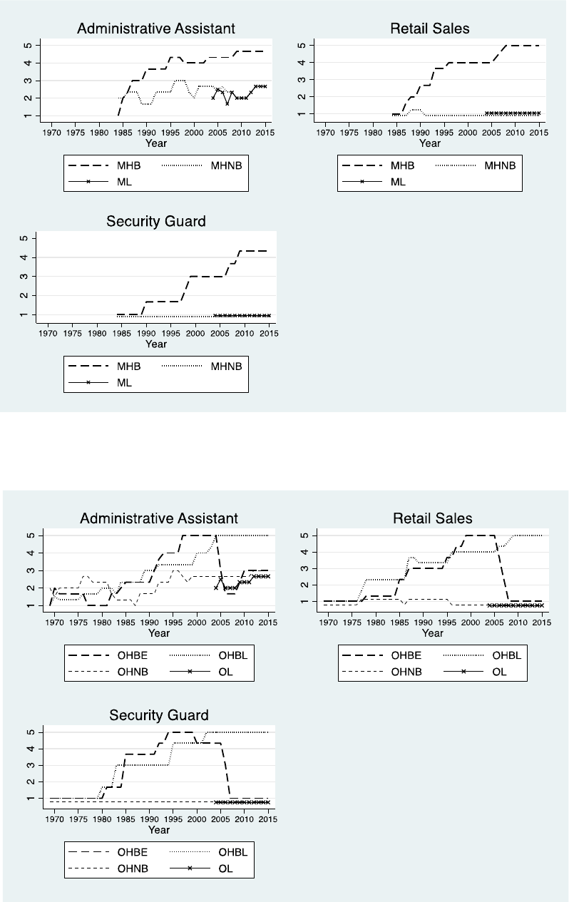
Appendix Figure A1: Job Responsibility Profiles for Middle-Age Resumes

Notes: See explanation in notes to Appendix Table A2.

Appendix Figure A2: Job Responsibility Profiles for Older Resumes

Notes: See explanation in notes to Appendix Table A2.