Informal Loans in Thailand: Stylized Facts and Empirical Analysis

Informal Loans in Thailand:

Stylized Facts and Empirical Analysis

Pim Pinitjitsamut

†

Rutgers University

Wisarut Suwanprasert

‡

Middle Tennessee State University

February 14, 2022

Abstract

This paper examines informal loans in Thailand using household survey data covering 4,800

individuals in 12 provinces across Thailand’s six regions. We proceed in three steps. First,

we establish stylized facts about informal loans. Second, we estimate the effects of household

characteristics on the decision to take out an informal loan and the amount of informal loan.

We ﬁnd that age, the number of household members, their savings, and the amount of existing

formal loans are the main factors that drive the decision to take out an informal loan. The main

determinations of the amount of informal loan are the interest rate, savings, the amount of

existing formal loans, the number of household members, and personal income. Third, we train

three machine learning models, namely K–Nearest Neighbors, Random Forest, and Gradient

Boosting, to predict whether an individual will take out an informal loan and the amount an

individual has borrowed through informal loans. We ﬁnd that the Gradient Boosting technique

with the top 15 most important features has the highest prediction rate of 76.46 percent, making

it the best model for data classiﬁcation. Generally, Random Forest outperforms the other two

algorithms in both classifying data and predicting the amount of informal loans.

Keywords: informal loans, machine learning, shadow economy, Thailand, loan sharks

JEL classiﬁcation numbers: E26, G51, O16, O17

The authors are grateful to the Department of Special Investigation (DSI), Ministry of Justice, Thailand, for kindly

sharing their data. This research was supported by Puey Ungphakorn Institute for Economic Research. All remaining

errors are ours.

†

Department of Economics, Rutgers University. Email: [email protected].

‡

Corresponding author. Department of Economics and Finance, Jennings A. Jones College of Business, Middle Ten-

nessee State University. Email: [email protected].

1 Introduction

In 2016, 88.1 percent of Thai households had debts totaling around 340,000 baht (approximately

$10,000), with informal loans accounting for 40.8 percent of these debts (Center for Economic and

Business Forecasting, UTCC). An Act of Parliament on legal lending rates for ﬁnancial institutions

has regulated interest rates on formal loans to no more than 25 percent per year. The annual

interest rates on informal loans, on the other hand, might reach 60 percent. (Siamwalla et al., 1990).

Because charging high interest rates on informal loans is unlawful, lenders are unable to sue for

nonpayment and therefore frequently exact payments through intimidation or physical assault.

A natural question is why households ﬁnance their expenditures with high-interest informal

loans rather than obtaining formal loans, with lower interest rates. If the cost of paying interest

were the only factor inﬂuencing a household’s decision to take out a loan, they would most likely

borrow from the formal sector. Therefore, the interest rate must not be the only factor driving the

decision.

This paper investigates the reasons why households take informal loans and the amount of

informal loans they take. We use household survey data from the Department of Special Inves-

tigation (DSI), Ministry of Justice, which cover around 4,800 households in 12 provinces across

Thailand’s six regions. Our analysis proceeds in three steps. First, we present stylized facts about

informal loans. Around 42.3 percent of individuals have an informal loan, with the average infor-

mal loan equal to 54,300 baht per person. We discover that among all occupations, government-

owned corporation (GOC) employees and government employees have the highest average infor-

mal loans. Around 28 percent of them use informal loans to repay existing debts, whereas around

53–60 percent of farmers, sellers, and business owners use informal loans for investments.

Second, we examine the effects of household characteristics on the decision to take out an

informal loan and the amount of informal loans. We use a Probit model, a Logit model, and a

linear probability model (LPM) to estimate the decision to take out an informal loan. We ﬁnd

that age, the number of household members, their savings, and the amount of existing formal

loans are the main factors. A larger household is more likely to take out an informal loan than a

small household does. A household that can borrow from the formal sector, or which has more

in savings, is less likely to borrow from the informal sector. We ﬁnd no evidence that personal

income inﬂuences this decision.

We then use linear models with ﬁxed effects to estimate the effects of household characteristics

on the amount of informal loans. The estimates suggest that the number of household members

and personal income are the main factors. On average, the amount of informal loans increases by

5% with each additional household member and increases by 0.3 percent for every one percent in-

crease in income. The empirical evidence indicates that the relationship is nonlinear. The marginal

effects suggest that the interest rate on informal loans, savings, and the amount of existing formal

loans all have a negative impact on the amount of informal loans.

Third, we use three machine learning techniques, namely K–Nearest Neighbors, Random For-

est, and Gradient Boosting, to classify whether or not a person will take an informal loan. The

results show that the Gradient Boosting method with the 15 most important features has the high-

est prediction rate of 76.46 percent, making it the best model for data classiﬁcation. Otherwise, the

Random Forest method outperforms the Gradient Boosting method in most cases. The ﬁve most

important features are total family expenses, total personal expenses, informal loan term, age, and

total income. Additionally, we use the models to predict the size of an informal loan each indi-

vidual will take out, based on socioeconomic factors. Random Forest is the best machine learning

approach for predicting the amount of an informal loan, since it has the lowest root mean square

error and the highest R-squared value.

The main contribution of this paper is to provide stylized facts and empirical analyses for

informal loans in Thailand. There are only a few studies on informal lending due to the lack

of data. Due to frequently unlawful high interest rates for informal loans, information on informal

loans is not disclosed to government authorities or established ﬁnancial institutions. This paper

is related to branches of study in the existing literature. In terms of research questions, our paper

is closely related to those of Siamwalla et al. (1990) and Tanomchat and Sampattavanija (2018), in

that these studies investigate aspects of informal loans in Thailand.

Siamwalla et al. (1990) reveal that throughout 1984 and 1985, 72.4 percent of the households

involved in borrowing activities received loans from the informal sector. Surprisingly, their analy-

sis suggests that the informal ﬁnancial market is competitive; the lenders did not have the market

power to extract economic rents from borrowers through high interest rates. Nevertheless, the

fact that informal loans are involved with high interest rates results from the economic rents from

information asymmetry among lenders. Karaivanov and Anke Kessler (2018) ﬁnd that informal

loans are related to interest rates lower than those for formal loans. Tanomchat and Sampattavanija

(2018) survey 694 households in Thailand and ﬁnd that informal interest rates correlate with the

lenders’ inﬂuence. They argue that high interest rates reﬂect the high default risks of debtors, and

only lenders who have inﬂuence, i.e., can use harassment or physical action, are willing to lend to

these debtors.

This paper is related to a group of studies that study the the effects of informal loans. Kislat

(2015) uses a difference-in-differences estimation to analyze the beneﬁts of informal lending among

different income groups of rural households in Northeast Thailand. Chemin (2008) uses a propen-

sity score estimation to study the effects on expenditure per capita, the supply of labor, and school

enrollment for children in Bangladesh. The beneﬁts of the government’s program on lending is in

Kaboski and Townsend (2005) and Pitt and Khandker (1998).

In addition, this paper is related to studies investigating the decision whether to borrow from

formal or informal ﬁnancial markets. In a study of informal lending in Peru, Guirkinger (2008)

ﬁnds that borrowers in the informal ﬁnancial market consist mainly of households without access

to the formal ﬁnancial market; the study also ﬁnds that household beneﬁt from lower transaction

costs in the informal ﬁncial market. Using a Probit model in Egypt, Moheldin and Wright (2000)

conclude that borrowers in the informal ﬁnancial market do not have the credit to access the formal

ﬁnancial market. Liu and Roth (2020) argue that informal-sector borrowers might ﬁnd themselves

in a debt trap, because lenders are motivated to keep them borrowing for an extended period.

The remainder of the paper is structured as follows. Section 2 provides background on the

situation in Thailand. Section 3 describes our data and variables. Section 4 summarizes stylized

facts. In Section 5 we estimate the effects of household characteristics on the decision to take out

an infomal loan and the amount of informal loan.. Section 6 shows the empirical analysis using

machine learning techniques. Section 7 concludes.

2 Background

In this paper, a loan is deﬁned as the amount of money received from an agent (lender), which

the recipient (borrower) is committed to repay in the future. Formal loans are loans provided by

formal organizations, including banks and ﬁnancial intermediaries. The Bank of Thailand and

the Ministry of Finance have imposed a ceiling on the interest rates charged on formal loans. For

example, the interest rates on personal loans cannot exceed 25 percent per year, and the credit card

interest rates cannot exceed 16 percent per year.

This paper focuses on informal loans, which are loans borrowed from unauthorized lenders.

Examples of such lenders include loan sharks, in-area investors, out-of-area investors, and stores.

The interest rates on informal loans, which are not under the supervision of the Bank of Thailand

and the Ministry of Finance, are often quoted as daily interest rates and exceed the legal cap on

interest rates. Generally, informal loans do not have a formal loan contract, because the interest

rates are illegally high, and so the loan contract would be nulliﬁed by law. However, the absence

of loan contracts makes informal loans more attractive to borrowers because of their ﬂexibility and

simplicity. Without a legal loan contract, lenders often have difﬁculties enforcing repayment, and

borrowers are not protected by law. Lenders may use social harassment or violence to enforce

repayment.

Informal loans may involve shadow contracts that seem legitimate but exploit a loophole in

the law. For example, a borrower may sign a loan contract to borrow 10,000 baht, with an interest

rate of 10 percent, but actually receive only 8,000 baht in cash. In this case, the contract is legally

binding, although the effective interest rate is illegally high.

To support borrowers who suffer from unjust informal loans, the Department of Special In-

vestigation (DSI) under the Ministry of Justice established the Legal Aid Center for Debtors and

Victims of Injustice (LADVIMOJ) in 2012. The main objective of the LADVIMOJ is to provide le-

gal advice to debtors who have informal loans with illegally high interest rates. The LADVIMOJ

reports that situations commonly arise from borrowers’ lack of knowledge of the legal system.

Borrowers are unfamiliar with formal loan contracts and do not have access to the justice system.

3 Data and Variable Description

3.1 Data Source

This study uses survey data from the Legal Aid Center for Debtors and Victims of Injustice (LAD-

VIMOJ), the Department of Special Investigation (DSI), Ministry of Justice. The data were, as

collected in 2014, funded by the LADVIMOJ.

The survey data is cross-sectional household-level data that consists of 4,878 households in

12 provinces across all six regions of Thailand. The provinces are Bangkok and Pathum Thani in

Bangkok metropolitan, Saraburi, Ratchaburi, and Phitsanulok in the Central region, Chonburi in

the Eastern region, Nakhon Si Thammarat and Songkhla in the Southern region, Chiang Rai in

the Northern region, Yasothon, Maha Sarakham, and Nong Khai in the Northeastern region. The

survey was conducted across 105 districts (Ampour) across Thailand.

The data contains information about loan takers and their families. That information includes

informal loan and formal loan amounts, interest rates, the type of informal loan lender, and the

purpose of informal loan. The dataset also contains socio-economics factors for Thai applicants,

such as age, gender, income, education level, and the expenditure level.

3.2 Variable Descripion and Cleaning Procedure

In the data, the unit of currency is the Thai baht. The exchange rate at the time of data collection

was approximately 33 baht to 1 USD. The main variables are the amount of formal and informal

loans and the interest rates. A formal loan is deﬁned as funds borrowed from registered banks. An

informal loan is deﬁned as funds received from non-banks that requires repayment in the future.

The interest rates on informal loans are quoted as monthly rates.

The survey categorizes occupation into nine groups: sellers, business owners, contract-based

workers, farmers, freelancers, private business employees, government-owned corporation em-

ployees, government employees, and unemployed.

We divide the reasons for taking formal and informal loans into four groups: (i) necessary, (ii)

unnecessary, (iii) investment, and (iv) debt repayment. Necessary reasons include hospital bills,

tuition fees, household expenses, and family traditional expenses. Unnecessary reasons include

mobile phone purchase, luxury gifts purchase, and others. Debt repayment means the repayment

of existing (formal and/or informal) loans.

We also group the sources of formal loans and informal loans. The sources of formal loans

are grouped into two types: banks and non-banks, where the bank group includes both private

and government banks, and the non-bank group includes ﬁnancial institutions, such as the Bank

for Agriculture and Agricultural Cooperatives. For informal loan sources, there are four groups:

in-area investors, out-of-area investors, loan sharks, and stores.

Total personal expense is constructed as the sum of a house mortgage, land rent, house rent,

food, utility bill, phone bill, tuition, transportation cost, investment, hospital bill, health and life

insurances, car payment, motorbike payment, phone bill, phone payment, and other costs.

Table 1: Statistical summary of the key variables

Summary Statistics Mean Median S.D. # of Obs

Amount of all loans 193,142.3 40,000 547,941.8 4,628

(total)

Amount of all loans 227,764.0 50,000 607,536.3 3,357

(conditional on having loan)

Amount of informal loans 22,961.7 0 105,505.9 4,628

(total)

Amount of informal loans 54,300.9 20,000 156,937.6 1,957

(conditional on having informal loans)

Interest rate on informal loans (percent) 16.5 10 63.4 1„957

Amount of formal loans 142,250.8 0 498,423.0 4,628

(total)

Amount of formal loans 297,083.4 80,000 687,696.7 2,216

(conditional on having formal loans)

Interest rate on formal loans (percent) 14.1 6 26.1 2216

Total family expenses 17,716.8 13,300 22,450.1 4,628

Total personal expenses 7,238.5 2,895 14,331.3 4,628

Total personal income 15,085.7 11,900 17,408.1 4,628

Personal savings 749.7 0 1,966.0 4,628

Last, we divide household occupations into two groups by income stream. The two groups

are occupations with monthly salaries and occupations with unstable income. After the process of

data cleaning, the total data consists of 4,623 observations.

4 Stylized Facts

4.1 Overview

Table 1 provides summary statistics for the main variables of interest.

Around 47.9 percent of individuals have formal loans, with an average of 297,000 baht per

person. Around 42.3 percent of individuals have an informal loan, with the average informal loan

equal to 54,300 baht per person. As a result, banks remain important ﬁnancial intermediaries in

the lending market.

The average monthly salary in our data is 15,085 baht. This is similar to the minimum monthly

income of 15,000 baht for college graduates. The minimum wage of workers with a high school

degree is 300 baht per day. Personal expenditures average 7,238 baht,while the average personal

savings is 749 baht. That is, personal expenditure is around 48 percent of total income.

4.2 Income and Consumption

Table 2 shows the average of personal income, consumption, and savings across different groups.

Chonburi and Saraburi have the highest average income, while Bangkok has the highest aver-

age living cost. Households save approximately 3 to 7 percent of their incomes. Saraburi, Nakhon

Si Thammarat, and Chonburi have higher savings than other provinces. An increase in level of

education is associated with higher income, more consumption, and larger saving.

The occupations are categorized into two groups; salary-based, and non-salary-based. The

average incomes these two occupation groups are 15,086 and 14,200 baht, respectively. Generally,

business owners, government employees, and government-owned corporation employees have a

relatively larger income. They consume and save more than the others do.

4.3 Informal Loans

This section documents the characteristics of individuals who have an informal loan.

Table 3 provides the average amount of informal loans in various age groups. With the assump-

tion that individuals in the working age range of 30–50 face higher expenses, such as personal and

family expenses, the amounts of informal loans taken out by those in this age range are expected

to be relatively larger than informal loans taken out by other age groups. Surprisingly, the average

amounts of informal loans are very similar across all age groups. There is no signiﬁcant difference

between ages. Therefore, the amount of informal loans might be determined by other factors apart

from age.

Table 3 also presents information on informal loans by each income group. Individuals with

no income have larger informal loans than those with incomes of 1–5,000 and 5,001–10,000. This

implies that informal loans can be used to smooth consumption. Individuals with incomes be-

tween 30,001 and 40,000 baht and 20,001 and 30,000 baht have the highest average informal loans,

of 135,853 baht and 105,007 baht, respectively. On the one hand, higher-income households do not

need to borrow money. Income, on the other hand, which indicates a household’s ability to repay

debts, permits the household to borrow more money.

The average informal loan amount for each occupation is shown in Table 4. Government em-

ployees and employees of government-owned corporations, in particular, have the highest average

informal loans, owing to the fact that they have the steadiest jobs, with better pay than others do.

Unemployed workers have an average informal loan amount of 53,849 baht. A lack of unemploy-

ment beneﬁts may have forced unemployed workers to take out informal loans to cover their daily

expenses. The average informal loan taken out by freelancers is three times less than that taken

out by unemployed workers.

Table 4 presents the average amount of loans in each province. Saraburi and Nakhon Si Tham-

marat, with average informal loans of 147,217 and 85,863 baht, respectively, have the largest av-

erage informal loans. The average informal loan in Pathum Thani is 9,461 baht, making it the

only province where the average informal loan is less than the average salary. Unfortunately, the

Table 2: The averages of income, consumption, and savings by location, education level, and oc-

cupation.

Income Consumption Savings

City/Rural Area

Bangkok Metropolitan 12,801.9 9,341.8 610.5

City 16,136.4 7,977.6 818.0

Rural 15,012.2 5,755.5 740.6

Province

Bangkok 15,140.0 13,537.4 473.2

Chonburi 18,547.1 6,966.0 1,060.9

Chiang Rai 14,565.1 1,853.5 282.3

Maha Sarakham 15,120.3 8,646.51 742.2

Nakhon Si Thammarat 16,642.2 11,542.1 1,598.4

Nong Khai 11,822.3 6,748.7 346.2

Pathum Thani 10,575.2 5,320.9 741.4

Phitsanulok 16,455.1 7,636.2 368.5

Ratchaburi 13,586.7 6,685.5 793.2

Saraburi 18,982.9 7,411.8 1,451.5

Songkhla 15,803.2 7,782.1 715.2

Yasothon 14,194.3 2,966.2 308.5

Education levels

No Education 13,735.5 5,816.9 325.4

Primary School 12,564.5 5,743.5 434.8

Middle School 14,619.4 7,499.9 801.5

High School 15,477.6 7,508.0 820.4

Associate Degree 15,851.0 8,283.1 822.4

Bachelor’s degree 22,303.1 10,380.3 1,490.4

Graduate Degree 32,805.6 14,224.3 3,097.6

Others 7,955.1 11,411.3 387.2

Types of Occupations

Salary Based 15,086.2 7,242.3 749.4

Non-Salary based 14,200.1 6,949.0 652.9

Occupations

Farmer 14,822.8 4,735.9 630.3

Seller 15,398.9 9,306.1 722.9

Freelancer 12,007.7 6,018.0 501.7

Contract based worker 9,851.6 4,438.1 397.5

Business owner 25,706.4 12,488.4 1,419.4

Private corporation employee 15,361.1 6,638.4 854.3

Government employee 21,726.5 10,127.6 1,412.7

Government-owned corporation employee 26,674.1 15,445.8 1,477.5

Unemployed 2,669.9 5,896.6 295.1

Table 3: Informal loans by age and by income range.

# of total

obs

Conditional on having an informal loan

# of obs Percent of

total obs

Mean Median S.D.

Total 4,628 1,957 42.3% 54,300.9 20,000 156,937.6

Age Range

<20 9 4 44.4% 8,750.0 6,500 8,301.6

20–24 145 50 34.5% 49,080.0 11,000 155,248.0

25–29 342 116 33.9% 67,422.7 17,500 370,403.7

30–34 419 171 40.8% 45,722.3 20,000 95,306.2

35–39 628 253 40.3% 63,060.1 20,000 184,293.6

40–44 720 314 43.6% 38,360.8 20,000 72,745.5

45–49 825 359 43.5% 52,078.6 20,000 102,731.2

50–54 717 313 43.7% 57,486.0 20,000 178,521.1

55–60 535 241 45.0% 66,387.0 20,000 131,914.7

>60 288 136 47.2% 54,780.6 20,000 100,995.6

Income Range

0 162 77 47.5% 48,962.3 11,500 131,747.6

1–5,000 414 176 42.5% 32,824.8 10,000 88,989.2

5,001–10,000 1,646 769 46.7% 25,435.9 10,000 51,991.3

10,001–20,000 1,646 627 38.1% 73,040.0 24,000 155,526.7

20,001–30,000 459 193 42.0% 105,007.1 40,000 305,319.9

30,001–40,000 124 49 39.5% 135,853.9 39,200 412,399.4

40,001–50,000 76 24 31.6% 89,916.7 42,500 113,606.8

50,001–100,000 88 39 44.3% 53,384.6 40,000 47,268.3

>100,000 13 3 23.1% 66,666.7 45,000 74,888.8

averages informal loans in other provinces are much greater than the average income.

Table 5 documents the interest rates on informal loans. The interest rates are relatively high for

loan sharks, at around 18.3 percent per month. Informal loans from in-area investors and out-of-

area investors have interest rates around 10–11 percent.

4.4 Reasons for Taking Out Informal Loans

Approximately 46.8% of individuals report that their informal loans are being used to cover nec-

essary expenses, while 41.5 percent report that their informal loans were utilized to support their

business. Only 9.4 percent of them use informal loans to repay existing debts and 2.3 percent of

them use loans to purchase unnecessary goods, such as luxury gifts and new phones.

Table 6 shows the most common reasons for taking out informal loans, by age group. As age

increases, the reason shifts from spending on necessary and unnecessary expenses to business

investment, while borrowing for debt rolling is relatively constant. Around 64 percent of young

Table 4: Informal loans by occupation and by province.

# of total

obs

Conditional on having an informal loan

# of obs Percent of

total obs

Mean Median S.D.

Total 4,628 1,957 42.3% 54,300.9 20,000 156,937.6

Occupation

Farmer 1,044 430 41.2% 90,818.4 30,000 149,445.4

Seller 1,245 652 52.4% 33,265.9 15,000 69,615.4

Freelancer 207 103 49.8% 18,713.6 10,000 54,295.7

Contract based worker 625 234 37.4% 31,776.9 14,000 79,521.4

Business owner 234 81 34.6% 65,432.1 20,000 132,670.4

Private corporation 745 275 36.9% 46,569.5 20,000 103,646.8

employee

Government employee 316 93 29.4% 117,932.0 30,000 459,845.8

Government-owned 69 22 31.9% 158,181.8 30,000 569,193.3

corporation employee

Unemployed 143 67 46.9% 53,849.3 10,000 140,558.7

Province

Bangkok 380 180 47.4% 29,207.8 13500 68,968.2

Chonburi 393 100 25.4% 64,167.0 20000 172,079.1

Chiang Rai 394 140 35.5% 46,239.3 27500 72,612.9

Maha Sarakham 394 125 31.7% 32,287.7 20000 38,317.4

Nakhon Si Thammarat 399 150 37.6% 85,863.3 30000 339,511.3

Nong Khai 412 219 53.2% 40,703.7 12000 157,563.7

Pathum Thani 401 217 54.1% 9,460.8 10000 6,733.7

Phitsanulok 320 73 22.8% 33,287.7 30000 31,070.9

Ratchaburi 395 207 52.4% 23,131.1 20000 17,964.5

Saraburi 405 245 60.5% 147,217.0 63250 183,584.1

Songkhla 352 119 33.8% 60,466.4 30000 102,323.7

Yasothon 383 182 47.5% 53,597.8 20000 211,717.9

borrowers use informal loans to spend on necessary expenses, while 16 percent borrow informal

loans to pay for unnecessary expenses. Only 14 percent borrow money for their business. A

majority of borrowers who use informal loans for unnecessary expenses are relatively young; only

1.7 percent of borrowers over the age of 30 use informal loans for unnecessary expenses.

The proportion of responders who report using informal loans to ﬁnance investment rises with

age, from 14.0 percent in the group ages 20 to 25 years old, to 56.8 percent in the group ages 55 to

60 years old. The proportion of responders in the necessary group is the highest between the ages

of 20 and 35, and decreases as age increases. The reason for this might be that people in their 20s

and 30s have large necessary expenses, such as tuition fees for themselves or their children, and

when they get older, their primary focus shifts toward running their own business.

Table 5: The averages of interest rates per month by lender types

# of Obs Percent Mean Median S.D.

In-area investor 537 27.4% 10.8 10 7.4

Out-of-area investor 610 31.2% 10.4 10 8.0

Loan sharks 590 30.1% 18.3 20 5.4

Store 220 11.2% 7.0 5 6.3

Total 1,957 100.0% 16.5 10 63.4

As the data shows a shift toward investment, the motivations for taking out informal loans

should be occupation-dependent. Therefore, we next investigate the reasons for making informal

loans, by occupation group.

Table 6 demonstrates that the reasons for taking out informal loans varies by occupation and

by province. In the aggregate, 46.8 percent of borrowers use informal loans to pay for necessary

expenses, and 41.5 percent of borrowers use informal loans to ﬁnance their business investments.

The fraction of borrowers who use informal loans for necessary expenses is relatively high for

private corporation employees (74.9 percent), freelancers (69.9 percent), contract-based workers

(69.7 percent), and the unemployed (65.7 percent), but it is relatively low for sellers (33.0 percent),

farmers (33.0 percent), and business owners (27.2 percent).

The proportion of borrowers who use informal loans for investments is relatively large for

farmers (60.0 percent), sellers (59.4 percent), and business owners (53.1 percent), and is relatively

small for freelancers (19.4 percent), contract-based workers (17.9 percent), and employees of pri-

vate corporations (8.0 percent). While 9.4 percent of individuals in the data use informal loans

mainly to repay existing debts, when categorized by occupation, it covers 27.3 percent of the em-

ployees of government-owned corporations and 28 percent of government employees. Only 6.3

percent of sellers and 5.6 percent of farmers use informal loans to repay existing debts.

Table 6 illustrates the breakdown of the reasons for taking out informal loans, by area. In

Bangkok and Pathum Thani, a substantial number of borrowers use informal loans to pay for

necessary expenditures. This might be due to the high cost of living in metropolitan areas. Informal

investment loans are used to ﬁnance a business by a signiﬁcant number of borrowers in Nong

Khai, Saraburi, Nakhon Si Thammarat, Chiang Rai, and Yasothorn. One possible reason is that

these provinces have metropolitan cities where business owners start their businesses and rural

areas where a majority of households are farmers.

4.5 From Who Did They Borrow Informal Loans?

Table 7 summarizes the sources of informal loans by age group, by occupation, and by province.

There is a consistent pattern in which out-of-area investors, loan sharks, and in-area investors each

cover around 30 percent of all loans. Less than 10 percent borrows from a store.

Around 35–44 percent of sellers, freelancers, contract-based workers, and business owners bor-

Table 6: Reasons for taking out informal loans by age, by occupation, and by province.

Investment Neccessary Pay off debt Unnecessary

Total

# of obs percent # of obs percent # of obs percent # of obs percent

Total 813 41.5% 916 46.8% 183 9.4% 45 2.3% 1,957

Age Range

<20 1 25.0% 3 75.0% 0 0.0% 0 0.0% 4

20–24 7 14.0% 32 64.0% 3 6.0% 8 16.0% 50

25–29 25 21.6% 70 60.3% 14 12.1% 7 6.0% 116

30–34 57 33.3% 101 59.1% 12 7.0% 1 0.6% 171

35–39 94 37.2% 117 46.2% 37 14.6% 5 2.0% 253

40–44 119 37.9% 162 51.6% 29 9.2% 4 1.3% 314

45–49 147 40.9% 175 48.7% 30 8.4% 7 1.9% 359

50–54 151 48.2% 126 40.3% 28 8.9% 8 2.6% 313

55–60 137 56.8% 83 34.4% 18 7.5% 3 1.2% 241

>60 75 55.1% 47 34.6% 12 8.8% 2 1.5% 136

Occupation

Farmer 258 60.0% 142 33.0% 24 5.6% 6 1.4% 430

Seller 387 59.4% 215 33.0% 41 6.3% 9 1.4% 652

Freelancer 20 19.4% 72 69.9% 10 9.7% 1 1.0% 103

Contract based worker 42 17.9% 163 69.7% 19 8.1% 10 4.3% 234

Business owner 43 53.1% 22 27.2% 15 18.5% 1 1.2% 81

Private corporation 22 8.0% 206 74.9% 35 12.7% 12 4.4% 275

employee

Government employee 22 23.7% 42 45.2% 26 28.0% 3 3.2% 93

Government-owned 5 22.7% 10 45.5% 6 27.3% 1 4.5% 22

corporation employee

Unemployed 14 20.9% 44 65.7% 7 10.4% 2 3.0% 67

Province

Bangkok 61 33.9% 100 55.6% 15 8.3% 4 2.2% 180

Chonburi 31 31.0% 54 54.0% 12 12.0% 3 3.0% 100

Chiang Rai 79 56.4% 45 32.1% 15 10.7% 1 0.7% 140

Maha Sarakham 59 47.2% 53 42.4% 8 6.4% 5 4.0% 125

Nakhon Si Thammarat 68 45.3% 68 45.3% 10 6.7% 4 2.7% 150

Nong Khai 97 44.3% 95 43.4% 24 11.0% 3 1.4% 219

Pathum Thani 64 29.5% 140 64.5% 13 6.0% 0 0.0% 217

Phitsanulok 29 39.7% 33 45.2% 9 12.3% 2 2.7% 73

Ratchaburi 85 41.1% 99 47.8% 8 3.9% 15 7.2% 207

Saraburi 123 50.2% 101 41.2% 18 7.3% 3 1.2% 245

Songkhla 28 23.5% 50 42.0% 40 33.6% 1 0.8% 119

Yasothon 89 48.9% 78 42.9% 11 6.0% 4 2.2% 182

Table 7: Types of lenders by age, by occupation, and by province.

In-area investor Out-of-area investor Loan sharks Store

Total

# of obs percent # of obs percent # of obs percent # of obs percent

Total 537 27.4% 610 31.2% 590 30.1% 220 11.2% 1,957

Age Range

<20 0 0.0% 0 0.0% 2 50.0% 2 50.0% 4

20–24 18 36.0% 17 34.0% 4 8.0% 11 22.0% 50

25–29 35 30.2% 46 39.7% 21 18.1% 14 12.1% 116

30–34 50 29.2% 57 33.3% 39 22.8% 25 14.6% 171

35–39 76 30.0% 71 28.1% 81 32.0% 25 9.9% 253

40–44 88 28.0% 88 28.0% 108 34.4% 30 9.6% 314

45–49 88 24.5% 114 31.8% 122 34.0% 35 9.7% 359

50–54 71 22.7% 89 28.4% 126 40.3% 27 8.6% 313

55–60 65 27.0% 86 35.7% 58 24.1% 32 13.3% 241

>60 46 33.8% 42 30.9% 29 21.3% 19 14.0% 136

Occupation

Farmer 141 32.8% 159 37.0% 85 19.8% 45 10.5% 430

Seller 164 25.2% 157 24.1% 254 39.0% 77 11.8% 652

Freelancer 22 21.4% 25 24.3% 45 43.7% 11 10.7% 103

Contract based worker 70 29.9% 61 26.1% 84 35.9% 19 8.1% 234

Business owner 24 29.6% 19 23.5% 28 34.6% 10 12.3% 81

Private corporation 48 17.5% 110 40.0% 74 26.9% 43 15.6% 275

employee

Government employee 40 43.0% 39 41.9% 6 6.5% 8 8.6% 93

Government-owned 5 22.7% 13 59.1% 1 4.5% 3 13.6% 22

corporation employee

Unemployed 23 34.3% 27 40.3% 13 19.4% 4 6.0% 67

Province

Bangkok 61 33.9% 86 47.8% 31 17.2% 2 1.1% 180

Chonburi 4 4.0% 42 42.0% 18 18.0% 36 36.0% 100

Chiang Rai 74 52.9% 35 25.0% 15 10.7% 16 11.4% 140

Maha Sarakham 54 43.2% 26 20.8% 23 18.4% 22 17.6% 125

Nakhon Si Thammarat 98 65.3% 23 15.3% 26 17.3% 3 2.0% 150

Nong Khai 28 12.8% 18 8.2% 151 68.9% 22 10.0% 219

Pathum Thani 4 1.8% 64 29.5% 144 66.4% 5 2.3% 217

Phitsanulok 14 19.2% 30 41.1% 15 20.5% 14 19.2% 73

Ratchaburi 58 28.0% 39 18.8% 67 32.4% 43 20.8% 207

Saraburi 57 23.3% 172 70.2% 14 5.7% 2 0.8% 245

Songkhla 28 23.5% 47 39.5% 13 10.9% 31 26.1% 119

Yasothon 57 31.3% 28 15.4% 73 40.1% 24 13.2% 182

row from loan sharks. Government employees and those at government-owned corporations usu-

ally borrow from out-of-area investors. Farmers borrow from both in-area and out-of-area in-

vestors.

Loan sharks are the most common lenders in Nong Khai and Pathum Thani, accounting for

roughly 66-69 percent of all loans. More than half of borrowers in Nakhon Si Thammarat (65.3

percent) and Chiang Rai (52.9 percent) borrow from in-area investors. Around 70 percent of indi-

viduals in Saraburi take out informal loans from out-of-area investors. Stores are the lenders for

36% of Chonburi borrowers.

5 Econometric Analysis

5.1 Methodology

We study the borrowing decision in two steps. First, we estimate the likelihood that a household

will take an informal loan, using a Probit model, a Logit model, and a linear probability model

(LPM). Second, we estimate factors that determine the amount of informal loans using OLS.

For the ﬁrst part, we estimate the following reduced-form equation:

Prob

(

informal loan

> 0

)

= β

+ β

age

Age

+ β

income

log

(

income

)

+ β

(

The number of household members

)

+ β

saving

log

(

saving

)

+ β

formal

log

(

formal loan

)

+ ε

, (1)

where Prob

(

informal loan

> 0

)

is the probability that household i takes an informal loan, Age

the age, log

(

income

)

is the logarithm of the income,

(

The number of household members

)

is the

number of household members, log

(

saving

)

is the logarithm of saving, log

(

formal loan

)

is the

logarithm of the amount of formal loan, and ε

is an error term.

We also consider the possibility of non-linearity by estimating the extended reduced-form

equation:

Prob

(

informal loan

> 0

)

= β

+ β

rate

(

Interest rate

)

+ β

rate

(

Interest rate

)

+ β

age

Age

+ β

age

Age

+ β

income

log

(

income

)

+ β

income

[

log

(

income

)]

+ β

(

The number of household members

)

+ β

saving

log

(

saving

)

+ β

saving

[

log

(

saving

)]

+ β

formal

log

(

formal loan

)

+ β

formal

[

log

(

formal loan

)]

+ X

β + ε

(2)

where the squares of

(

Interest rate

)

, Age

, log

(

income

)

, log

(

saving

)

, and log

(

formal loan

)

are

included.

Next, we investigate the determinants of the amoung of informal loan. We estimate the follow-

ing reduced-form equation:

log

(

informal loan

)

= β

+ β

rate

(

Interest rate

)

+ β

age

Age

+ β

income

log

(

income

)

+ β

(

The number of household members

)

+ β

saving

log

(

saving

)

+ β

formal

log

(

formal loan

)

+ X

β + ε

, (3)

where log

(

informal loan

)

is the logarithm of the amount of informal loan. The additional ex-

planatory variables are the interest rate on the loan, denoted by

(

Interest rate

)

, and the vector of

controls, denoted by X

. The controls are gender ﬁxed effects, province ﬁxed effects, education-

level ﬁxed effects, occupation ﬁxed effects, and status-in-household ﬁxed effects.

To allow for the possibility of non-linear relationship, we extend the baseline model to

log

(

informal loan

)

= β

+ β

rate

(

Interest rate

)

+ β

rate

(

Interest rate

)

+ β

age

Age

+ β

age

Age

+ β

income

log

(

income

)

+ β

income

[

log

(

income

)]

+ β

(

The number of household members

)

+ β

saving

log

(

saving

)

+ β

saving

[

log

(

saving

)]

+ β

formal

log

(

formal loan

)

+ β

formal

[

log

(

formal loan

)]

+ X

β + ε

, (4)

where the squares of

(

Interest rate

)

, Age

, log

(

income

)

, log

(

saving

)

, and log

(

formal loan

)

are

included.

5.2 Empirical Results

We estimate equations (1) and (2) using three different models: a Probit model, a Logit model, and

a linear probability model, and report the coefﬁcients and corresponding marginal effects in Tables

The reported standard errors are heteroskedasticity-robust standard errors. We ﬁnd that the

number of age, household members, their savings, and the amount of existing formal loans are

important determinants. The coefﬁcient of age is statistically signiﬁcant from zero in the Probit

and Logit models but is not in the linear probability model. Based on the Probit and Logit models,

when age increases by 10 years, the probability of taking out an informal loan increases by 2.3

percent.

A larger household is more likely to take out an informal loan than a small household does. A

household that can borrow from the formal sector or have a larger saving is less likely to borrow

from the informal sector. We do not ﬁnd evidence that personal income inﬂuences the decision.

Columns (6)–(11) show empirical results when the squared terms are included. Only the effect

of age is non-monotonic. The marginal effect of age at the means has a similar magnitude to the

Table 8: The choice of taking out an informal loan

Probit Logit LPM Probit Logit LPM

coef. marginal coef. marginal coef. coef. marginal coef. marginal coef. marginal

Variables (1) (2) (3) (4) (5) (6) (7) (8) (9) (10) (11)

Age 0.00610*** 0.00235*** 0.00983*** 0.00235*** -0.000995 0.0281*** 0.00243*** 0.0454*** 0.00244*** 0.000600 -0.000969

(0.00168) (0.000646) (0.00271) (0.000645) (0.000822) (0.0102) (0.000646) (0.0165) (0.000646) (0.00421) (0.000846)

Age

-0.000245** -0.000396** -1.77e-05

(0.000112) (0.000180) (4.45e-05)

log

(

income

)

-0.00803 -0.00309 -0.0127 -0.00304 -0.00753 -0.0190 -0.00298 -0.0313 -0.00274 -0.0225 0.000800

(0.0102) (0.00394) (0.0164) (0.00393) (0.00564) (0.0365) (0.0106) (0.0588) (0.0105) (0.0166) (0.0113)

[

log

(

income

)]

0.000619 0.00109 0.00129

(0.00333) (0.00535) (0.00139)

The number of 0.0348*** 0.0134*** 0.0560*** 0.0134*** 0.00214 0.0335*** 0.0129*** 0.0539*** 0.0129*** 0.00213 0.00213

household members (0.0121) (0.00463) (0.0193) (0.00460) (0.00505) (0.0121) (0.00465) (0.0194) (0.00462) (0.00506) (0.00506)

log

(

saving

)

-0.0168*** -0.00646*** -0.0272*** -0.00649*** -0.00797*** -0.0271 -0.00709** -0.0433 -0.00713** -0.00876 -0.00829***

(0.00557) (0.00214) (0.00897) (0.00214) (0.00222) (0.0270) (0.00305) (0.0433) (0.00307) (0.0108) (0.00312)

[

log

(

saving

)]

0.00150 0.00235 7.97e-05

(0.00362) (0.00581) (0.00143)

log

(

formal loan

)

-0.0246*** -0.00946*** -0.0396*** -0.00946*** -0.00470*** 0.0144 -0.00764*** 0.0238 -0.00753*** -0.00539 -0.00488***

(0.00327) (0.00123) (0.00526) (0.00123) (0.00137) (0.0199) (0.00151) (0.0324) (0.00153) (0.00751) (0.00152)

[

log

(

formal loan

)]

-0.00324** -0.00528** 4.67e-05

(0.00164) (0.00268) (0.000616)

Observations 4,628 4,628 4,628 4,628 4,628 4,628 4,628 4,628 4,628 4,628 4,628

Adjusted R-squared 0.0153 0.0153 0.0773 0.0167 0.0167 0.0767

Note: Only the linear probability model on columns (5) and (11) includes ﬁxed effects for gender, province, education level, occupation,

and the status in the household. *,**, and *** indicate the signiﬁcance level of 0.10, 0.05, and 0.01, respectively.

marginal effect estimated from the linear model.

Table 9 presents estimates of Equations (3) and (4). When we include additional square terms,

we ﬁnd that the effects on the amount of informal loans are non-linear. This ﬁnding is consistent

with the statistics in Table 3 that the amount of informal loan is non-monotonic in the income

range. Therefore, we provide the marginal effects at the means for estimates on column (3).

The amount of informal loan is concave in age and is convex in income, saving, and the amount

of formal loan. The amount of informal loans is increasing in income and the number of household

members, and decreasing in saving and the amount of formal loans. On average, the amount

of informal loans increases by 5% with each additional household member and increases by 0.3

percent for every one percent increase in income.

Generally, a larger household has a larger informal loan than a smaller household does. A

10-percent increase in saving increases the amount of informal loan by 3.2 percent. A 10-percent

increase in the amount of formal loan raises the amount of informal loan by 0.1 percent. The

coefﬁcient of age is not statistically different from zero and its magnitude is negligible. This is

consistent with Table 3 that the amounts of informal loans across age groups are approximately

equal.

Table 10 compares the borrowing behavior between genders. Columns (1) and (2) show the

estimates when the observations are restricted to male, and Columns (3) and (4) show the estimates

when the observations are restricted to female. Men are more sensitive to a change in interest rate

and income than women do. When the interest rate on informal loans increases by one percentage

point, men’s informal loans decrease by 3.7 percent while women’s informal loans decrease by

2.4 percent. The effect of income among male is more convex than the effect of income among

females. At the means, the marginal effect of income is larger among males. On average a 10-

percent increase in income raises informal loan of a man by 4.2 percent and raises informal loan of

a woman by 2.2 percent. Women’s informal loans respond to the number of household members

and the amount of formal loan, but men’s informal loans do not. A woman that has one additional

household member tends to borrow informal loan more by around 0.06 percent. The effect of

saving of male is more convex than the effect of saving of female. At the means, the marginal

effects of saving of males and females are 0.0061 and -0.0580, respectively. The effects of age and

the amount of formal loans are negligible for both genders.

We then consider heterogeneity across occupations. We classify occupations into groups based

on the nature of the occupation: government jobs, private jobs, and the unemployed. Government

jobs include government employees and government-owned corporation employees. Private jobs

are divided into ﬁxed-income jobs and ﬂexible-income jobs. Fixed-income jobs are private busi-

ness employees. Flexible-income jobs include sellers, business owners, contract-based workers,

farmers, and freelancers.

Table 11 summarizes the estimates by occupational group. The effect of age is statistically

signiﬁcant only among the ﬂexible-income private employees. The marginal effect of interest rate

is in a similar range across all occupation. However, the standard errors of the marginal effect

Table 9: The determinants of the amount of informal loan, log

(

informal loan

)

Equation (3) Equation (4)

coef. coef. marginal

Variables (1) (2) (3)

Interest rate -0.0661** -3.112*** -3.011***

(0.0335) (0.430) (0.416)

(

Interest rate

)

0.305***

(0.0428)

Age 0.00502 0.0474** 0.00395

(0.00320) (0.0193) (0.00313)

Age

-0.000483**

(0.000206)

log

(

income

)

0.132*** -0.211*** 0.287***

(0.0258) (0.0645) (0.0403)

[

log

(

income

)]

0.0276***

(0.00512)

The number of 0.0577*** 0.0499*** 0.0499***

household members (0.0190) (0.0186) (0.0186)

log

(

saving

)

0.0228*** -0.156*** -0.0322**

(0.00880) (0.0410) (0.0133)

[

log

(

saving

)]

0.0231***

(0.00554)

log

(

formal loan

)

0.0119** -0.117*** -0.0153*

(0.00550) (0.0334) (0.00810)

[

log

(

formal loan

)]

0.0108***

(0.00285)

Observations 1,957 1,957 1,957

R-squared 0.279 0.336

Adjusted R-squared 0.263 0.320

Note: All regressions include ﬁxed effects for gender, province, education level, occupation, and

the status in the household. *,**, and *** indicate the signiﬁcance level of 0.10, 0.05, and 0.01,

respectively.

Table 10: The determinants of the amount of informal loan, log

(

informal loan

)

, by gender

Male Female

coef. marginal coef. marginal

Variables (1) (2) (3) (4)

Interest rate -3.836*** -3.737*** -2.468*** -2.377***

(0.633) (0.616) (0.573) (0.552)

(

Interest rate

)

0.376*** 0.242***

(0.0627) (0.0571)

Age 0.0362 0.00614 0.0503** 0.00300

(0.0345) (0.00504) (0.0230) (0.00414)

Age

-0.000331 -0.000529**

(0.000372) (0.000240)

log

(

income

)

-0.428*** 0.417*** -0.0916 0.223***

(0.106) (0.0839) (0.0776) (0.0444)

[

log

(

income

)]

0.0453*** 0.0179***

(0.00910) (0.00602)

The number of -0.00141 -0.00141 0.0590*** 0.0590***

household members (0.0371) (0.0371) (0.0217) (0.0217)

log

(

saving

)

-0.198*** 0.00607 -0.140** -0.0580***

(0.0648) (0.0152) (0.0571) (0.0225)

[

log

(

saving

)]

0.0321*** 0.0174**

(0.00881) (0.00773)

log

(

formal loan

)

-0.0660 -0.0144 -0.146*** -0.0119

(0.0495) (0.0117) (0.0433) (0.0110)

[

log

(

formal loan

)]

0.00529 0.0146***

(0.00415) (0.00370)

Observations 784 784 1,171 1,171

R-squared 0.446 0.271

Adjusted R-squared 0.414 0.241

Note: All regressions include ﬁxed effects for province, education level, occupation, and the status

in the household. *,**, and *** indicate the signiﬁcance level of 0.10, 0.05, and 0.01, respectively.

Table 11: The determinants of the amount of informal loan, log

(

informal loan

)

, by occupation type

Government Private Unemployed

ﬁxed-income ﬂexible-income

coef. marginal coef. marginal coef. marginal coef. marginal

Variables (1) (2) (3) (4) (5) (6) (7) (8)

Interest rate -2.636 -2.540 -2.238*** -2.143*** -3.510*** -3.428*** -1.745 -3.349

(2.248) (2.172) (0.638) (0.610) (0.608) (0.594) (5.620) (3.773)

(

Interest rate

)

0.281 0.220*** 0.353*** -5.079

(0.223) (0.0632) (0.0605) (7.268)

Age -0.0904 0.00579 -0.00375 -0.00226 0.102*** 0.00977** 0.0450 0.0117

(0.0780) (0.0200) (0.0304) (0.00451) (0.0267) (0.00472) (0.0765) (0.0161)

Age

0.00115 1.62e-05 -0.00104*** -0.000331

(0.000784) (0.000311) (0.000296) (0.000799)

log

(

income

)

2.915 0.392 -0.00796 0.259*** -0.217 0.332*** 0.368 0.258

(5.923) (0.297) (0.110) (0.0623) (0.212) (0.0615) (0.404) (0.282)

[

log

(

income

)]

-0.129 0.0146* 0.0295** -0.0387

(0.300) (0.00827) (0.0125) (0.0434)

The number of 0.0426 0.0426 0.0480** 0.0480** 0.0111 0.0111 0.130 0.130

household members (0.0853) (0.0853) (0.0239) (0.0239) (0.0284) (0.0284) (0.0934) (0.0934)

log

(

saving

)

0.185 0.0345 -0.0726 -0.0396 -0.204*** -0.0190 0.0970 0.0519

(0.182) (0.0412) (0.0774) (0.0382) (0.0543) (0.0125) (0.319) (0.167)

[

log

(

saving

)]

-0.0188 0.00875 0.0272*** -0.0138

(0.0248) (0.0107) (0.00741) (0.0500)

log

(

formal loan

)

-0.147 0.0912 -0.192*** -0.0626*** -0.0790* -0.0121 -0.393 -0.0691

(0.141) (0.0755) (0.0537) (0.0232) (0.0478) (0.00829) (0.356) (0.139)

[

log

(

formal loan

)]

0.0126 0.0192*** 0.00611 0.0401

(0.0111) (0.00462) (0.00401) (0.0273)

Observations 113 113 883 883 889 889 66 66

R-squared 0.389 0.227 0.461 0.702

Adjusted R-squared 0.134 0.196 0.435 0.446

Note: All regressions include ﬁxed effects for gender, province, education level, and the status in the household. *,**, and *** indicate the signiﬁcance

level of 0.10, 0.05, and 0.01, respectively.

of interest rate in the case of ﬁxed-income and ﬂexible income private employees are 0.61 and

0.60, respectively, while the standard errors of interest rates in the case of government employees,

and the unemployed are 2.17 and 3.77, respectively. The marginal effect of interest rate is -2.14 for

ﬁxed-income private employees, -3.43 for ﬂexible-income private employees, -2.54 for government

employees, and -3.35 for the unemployed. Age matters only among the group of ﬁxed-income

private employees.

At the means, the marginal effects of income of government employees and private employees

are similar. However, the effect of income is convex among private employees (both ﬁxed-income

and ﬂexible-income), but it is concave among government employees. Saving only matters for

ﬂexible-income private employees. The amount of formal loan affects the amount of informal loan

for ﬁxed-income private employees.

Table 12 displays the results by region. The effect of interest rate is sizable in the Central, the

Eastern, the Southern, and the Northeastern. Income is the only factor that affects the amount of

loans in all regions. The marginal effect of income at the means is positive in all regions except the

Eastern. The marginal effect of income is 0.19 in the Bangkok metropolitan area, 0.41 in the Central,

-0.61 in the Eastern, 0.39 in the Southern, 0.19 in the Northern, and 0.275 in the Northeastern.

Saving has a substantial impact on the amount of informal loan in the Central and the Eastern.

Table 13 summarizes the factors that inﬂuence the amount of informal loans by household

status. Interest rate, age, income, savings, and the amount of formal loan all affect the amount of

informal loan for household heads. The interest rate has an effect on the amount of formal loans

taken out by household heads and their spouses only. Income affects the amount of informal loan

only among household heads, the spouses, and the children. For parents of the household heads

and other relatives, none of the coefﬁcients are statistically signiﬁcant from zero.

6 Machine Learning

In this section, we use machine learning techniques to determine the characteristics essential to

predicting a household’s decision whether to take out an informal loan and the amount of such an

informal loan.

6.1 Methodology

Our data contains two types of variables: numerical variables and categorical variables. Numerical

variables are the number of members in the household, the number of members with income, the

number of members in college, the number of unemployed members, the number of stay-at-home

members, gender, age, the number of members with a second job, total income, total personal

expenditure, total family expenditure, savings, amount of informal loan, amount of formal loan,

outstanding balance of formal loan, formal loan interest, informal loan term, and informal loan

interest rate. Categorical variables are the status of the individual in the household, province,

Table 12: The determinants of the amount of informal loan, log

(

informal loan

)

, by region

Bangkok metro. Central Eastern Southern Northern Northeastern

coef. marginal coef. marginal coef. marginal coef. marginal coef. marginal coef. marginal

Variables (1) (2) (3) (4) (5) (6) (7) (8) (9) (10) (11) (12)

Interest rate -2.648 -1.436 -3.045*** -2.915*** -7.022** -4.256*** -3.086** -2.996** 1.156 -1.106 -12.43*** -1.365

(2.960) (1.380) (0.655) (0.627) (3.041) (1.554) (1.277) (1.236) (10.02) (4.226) (4.298) (0.982)

(

Interest rate

)

3.124 0.302*** 12.72 0.274** -16.49 41.92**

(5.331) (0.0649) (8.338) (0.126) (43.02) (17.08)

Age 0.0393 0.00379 0.0568* -0.000202 0.0176 0.0232* 0.111 0.0125 0.0697 -0.00877 0.000741 -0.00100

(0.0387) (0.00635) (0.0307) (0.00536) (0.0633) (0.0127) (0.0860) (0.0132) (0.0653) (0.0110) (0.0404) (0.00612)

Age

-0.000401 -0.000628* 7.27e-05 -0.00115 -0.000871 -1.83e-05

(0.000445) (0.000323) (0.000754) (0.000923) (0.000714) (0.000406)

log

(

income

)

-0.00893 0.194*** -0.594*** 0.412*** -11.10*** -0.613** -0.381* 0.390** 0.687 0.193* -0.117 0.275***

(0.0927) (0.0660) (0.105) (0.0831) (3.284) (0.244) (0.199) (0.170) (1.298) (0.104) (0.165) (0.0696)

[

log

(

income

)]

0.0120 0.0541*** 0.557*** 0.0419** -0.0267 0.0219*

(0.00841) (0.00943) (0.170) (0.0190) (0.0705) (0.0113)

The number of -0.00505 -0.00505 -0.0222 -0.0222 0.229* 0.229* 0.156** 0.156** 0.100 0.100 0.103** 0.103**

household members (0.0244) (0.0244) (0.0365) (0.0365) (0.119) (0.119) (0.0607) (0.0607) (0.0664) (0.0664) (0.0414) (0.0414)

log

(

saving

)

0.126 0.0656 -0.138** 0.0642*** -0.367** -0.105 -0.0955 -0.00780 -0.242* 0.0228 -0.0841 -0.0582

(0.115) (0.0602) (0.0700) (0.0176) (0.174) (0.0643) (0.128) (0.0485) (0.137) (0.0510) (0.102) (0.0611)

[

log

(

saving

)]

-0.0173 0.0236*** 0.0456** 0.0177 0.0321 0.00880

(0.0161) (0.00908) (0.0211) (0.0170) (0.0195) (0.0142)

log

(

formal loan

)

0.0133 0.0203 -0.167*** 0.00570 0.0119 0.00570 -0.127 0.00426 -0.0461 -0.0273 -0.181*** -0.0129

(0.0883) (0.0634) (0.0551) (0.00849) (0.123) (0.0497) (0.116) (0.0160) (0.105) (0.0375) (0.0662) (0.0169)

[

log

(

formal loan

)]

0.00217 0.0144*** -0.000782 0.0121 0.00125 0.0179***

(0.00799) (0.00462) (0.00972) (0.00999) (0.00897) (0.00554)

Observations 393 393 524 524 98 98 267 267 138 138 523 523

R-squared 0.269 0.522 0.585 0.271 0.264 0.207

Adjusted R-squared 0.213 0.488 0.416 0.167 0.0755 0.154

Note: All regressions include ﬁxed effects for gender, education level, occupation, and the status in the household. *,**, and *** indicate the signiﬁcance level of 0.10, 0.05, and 0.01,

respectively.

Table 13: The determinants of the amount of informal loan, log

(

informal loan

)

, by the status in the household

Head of HH Spouse Children Parents Other

coef. marginal coef. marginal coef. marginal coef. marginal coef. marginal

Variables (1) (2) (3) (4) (5) (6) (7) (8) (9) (10)

Interest rate -3.355*** -3.251*** -2.254*** -2.174*** -1.580 -1.524 -5.956 -7.791* -2.456 -4.424

(0.559) (0.542) (0.776) (0.749) (3.392) (3.246) (17.77) (4.302) (16.01) (10.95)

(

Interest rate

)

0.334*** 0.222*** 0.130 -9.120 -7.716

(0.0555) (0.0769) (0.338) (80.38) (21.46)

Age 0.0836*** 0.00818** 0.0282 -0.000920 -0.0719 -0.00745 0.0382 -0.0235 0.106 0.0166

(0.0258) (0.00399) (0.0316) (0.00517) (0.164) (0.0330) (0.338) (0.0377) (0.117) (0.0601)

Age

-0.000807*** -0.000333 0.00107 -0.000609 -0.000911

(0.000275) (0.000345) (0.00234) (0.00330) (0.00136)

log

(

income

)

-0.240** 0.306*** -0.0860 0.212*** -0.955*** 0.644*** 0.0412 0.370 -0.612 -0.0618

(0.0939) (0.0607) (0.107) (0.0563) (0.314) (0.227) (0.773) (0.566) (1.077) (0.519)

[

log

(

income

)]

0.0294*** 0.0169** 0.102*** 0.0197 0.0346

(0.00733) (0.00804) (0.0337) (0.0769) (0.0923)

The number of 0.00412 0.00412 0.113*** 0.113*** 0.0726 0.0726 0.286 0.286 0.125 0.125

household members (0.0224) (0.0224) (0.0280) (0.0280) (0.126) (0.126) (0.315) (0.315) (0.283) (0.283)

log

(

saving

)

-0.184*** -0.0246 -0.0866 -0.0406 -0.203 -0.0267 -0.847 -0.294 1.174 0.387

(0.0574) (0.0165) (0.0647) (0.0250) (0.209) (0.0671) (0.584) (0.251) (1.056) (0.378)

[

log

(

saving

)]

0.0279*** 0.00969 0.0275 0.128 -0.172

(0.00774) (0.00892) (0.0296) (0.0823) (0.151)

log

(

formal loan

)

-0.139*** -0.0318** -0.103* 0.00216 0.0298 0.0480* 0.124 0.00601 -0.508 -0.178

(0.0524) (0.0127) (0.0564) (0.0139) (0.182) (0.0277) (0.657) (0.0627) (1.323) (0.506)

[

log

(

formal loan

)]

0.0117*** 0.0114** 0.00140 -0.0103 0.0435

(0.00451) (0.00484) (0.0144) (0.0580) (0.108)

Observations 1,084 1,084 694 694 89 89 40 40 37 37

R-squared 0.430 0.268 0.473 0.667 0.950

Adjusted R-squared 0.410 0.227 0.108 0.00173 0.405

Note: All regressions include ﬁxed effects for gender, education level, occupation, and region. *,**, and *** indicate the signiﬁcance level of 0.10, 0.05, and 0.01, respectively.

education level, occupation, the reason for taking formal loans, and the reason for taking informal

loans.

We use log-transformation on total income, savings, outstanding balance of formal loan, total

personal expenditure, and total family expenditure. All numerical variables are standardized by

removing the mean and scaling to unit variance. The standard score of samples is calculated as a

normal distribution (z–score). We create dummy variables for categorical variables using one-hot

encoding.

For the classiﬁcation process, we use supervised machine learning models: K–Nearest Neigh-

bor (KNN), Random Forest, and Extreme Gradient Boosting (XGBoost). We rank features both

numerical and categorical using Random Forest importance feature selection. This selection sorts

variables based on the magnitude of their effects on the target variable. In decision trees, every

node is a condition of how to split values in a single feature, so that similar values of the depen-

dent variable end up in the same set after the split. For classiﬁcation problems, the condition is

based on Gini impurity, while for regression trees, it is based on variance. With the training set,

we compute how much each feature contributes to averaging the decrease in impurity over trees.

We use two sets of features. The ﬁrst set, denoted by Dataset 1, includes all variables, and the

second set, denoted by Dataset 2, excludes the reason for taking an informal loan, because it is not

publicly available information for government agencies or policymakers. At the beginning of the

classiﬁcation process, we split the dataset into testing and training sets, where we use a test size of

0.4, so the models have larger amounts of data to train on, and we use the random state of 23.

Our ﬁrst machine learning technique is K–Nearest Neighbors. It is an algorithm that classiﬁes

objects based on the nearest training examples into several classes, to forecast the classiﬁcation of a

new sample point. With a dataset, the distance between each unknown sample will be calculated.

The unknown sample may be classiﬁed based on the distance with the smallest value to sample in

the training set.

Second, Random Forest classiﬁcation is an ensemble tree-based learning algorithm, where the

RF classiﬁer is a set of decision trees from randomly selected subsets of the training set. It aggre-

gates the votes from different decision trees to decide the ﬁnal class of the test object. Similarly, we

split the train and test dataset by the ratio of 40 percent for the test set and 60 percent for the train

set. We set 150 trees in the forest for Random Forest classiﬁcation.

Last, XGBoost is a decision-tree based ensemble using a Gradient Boosting framework. We use

the XGBoost model for classiﬁcation with the default setup for the ﬁrst setup. We set the maximum

depth of 8, the learning rate of 0.1 and the subsample of 0.5 for second setup. For our third setup

we use hyperparameter tuning by using grid search. Finally, for our fourth setup, we use Gamma

XGBoost tuning.

Table 14: The ranking of features

Ranking Dataset 1 Dataset 2

1 Total family expenses Total family expenses

2 Informal loan interest Informal loan interest

3 Age Total personal expenses

4 Total personal expenses Age

5 Informal loan term Total income

6 Total income Informal loan term

7 Amount of formal loan Amount of formal loan

8 Number of family member Number of family member

9 Savings Savings

10 Formal loan interest rate Formal loan interest rate

11 Number of family members with income Number of family members with income

12 Number of family members with education Number of family members with education

13 Reason - Investment Gender

14 Gender Province - Saraburi

15 Occupation - Seller Occupation - Seller

6.2 Results

6.2.1 Correlation plot and feature ranking

The ranking is shown in Table 14. The top 15 most important features from Dataset 2 are total fam-

ily expenditure, informal loan interest rate, total personal expenditure, age, total income, informal

loan term, amount of formal loan, number of members in household, savings, formal loan interest,

number of members with income, number of members with education, gender, living in Saraburi,

and occupation as seller.

The correlation plot in Figure 1 shows us the linear relationship between each variable. With

the ﬁeld, we need to check for features of multicollinearity because this will affect the relationship

with our independent variables. We can see that a few variables are highly correlated with each

other. The number of household members is associated with the number of members in college and

the number of members with income. Moreover, there is a correlation of 0.73 between the amount

of the formal loans and the formal loan interest rate. Figure 1 also shows that saving is negatively

correlated with occupation as a seller. This can imply that sellers might have lesser savings than

other occupations. At the same time, occupation as a seller also has a negative correlation with the

amount of the formal loan. This along with Table 14 can imply that sellers have difﬁculty taking

formal loans. The causes could be that sellers have unstable income and lesser savings or assets

than other occupations, thus they tend to resort to borrowing an informal loan.

Table 14 represents that the most crucial factor that plays a role in an individual taking an infor-

mal loan is total family expenses. Often, families with high costs are likely to take out an everyday

loan to cover the expenditure that exceeds their incomes. Moreover, the ranking of importance

Table 15: The classiﬁcation result comparison

Regression Models Data #features R

Score RMSE Classiﬁcation Accuracy Rate

K–Nearest Neighbors

All 0.3502 0.3920 67.07%

Top 15 0.3466 0.3931 72.83%

All 0.3502 0.3920 66.98%

Top 15 0.3423 0.3944 69.56%

Random Forest

All 0.5137 0.3391 75.90%

Top 15 0.4837 0.3494 74.90%

All 0.5042 0.3424 75.10%

Top 15 0.4873 0.3482 74.10%

Gradient Boosting

All 0.4645 0.3559 73.93%

Top 15 0.465 0.3557 76.46%

All 0.4526 0.3598 74.98%

Top 15 0.4721 0.3533 73.16%

features also demonstrates that households that live in Saraburi and head of household occupa-

tion are sellers tend to have a higher chance of taking out informal loans. The reason can be that

sellers have relatively more uncertainty in terms of income and investment. The inventory is vari-

ous monthly and their incomes. Thus, the chance that the head of household with this occupation

will take out informal loans is higher than other occupations. Even though the freelancer may face

similar uncertainty, the monthly investment paid in advance is required to tend to be lesser than

sellers. With other features, it is difﬁcult to determine the household that need assistance from the

government on loan issue because of a limitation in data. For example, not all household with high

total family expenses are likely to takeout informal loan, unless the household expenses overly ex-

ceed their income. However, one of the features that might be interested for policy maker is the

occupation as seller and household that live in Saraburi. They can focus on helping people with

occupation as seller to mitigate the amount of informal loan taken in economy and investigate the

reasons why households that live in Saraburi has higher the likelihood of them taking informal

loans than households that live in other provinces.

6.2.2 Classiﬁcation

For each machine learning technique, we do four experiments, , which combine two possible

datasets and two different numbers of features. Dataset 1 has all the variables, and Dataset 2

excludes information on the reason for taking an informal loan. For each dataset, we run two

experiments: one with all features and one with only the top 15 features.

We compare the performance of the machine learning techniques by using their classiﬁcation

accuracy rates. A classiﬁcation accuracy rate measures the accuracy with which the model predicts

whether a person will take out an informal loan. Table 15 describes the classiﬁcation accuracy rates

of all 12 experiments.

In three of four experiments, Random Forest has the highest classiﬁcation accuracy rates. Among

the four XGBoost setups, the Grid search setup is the best for Dataset 1 when using all features,

and the setup using Gamma XGBoost tuning is the best in the other three experiments. When com-

pared to the other two machine learning models, the K–Nearest Neighbors method has the lowest

classiﬁcation accuracy rate among all four models.

In terms of predictive power, the best model is Gradient Boosting, with grid search, using the

top 15 features in the dataset, with the reason for borrowing informal loans.

6.2.3 Predicting informal loans

After the classiﬁcation models, we examine how features can predict the amount each person will

borrow using informal loans. Table 15 summarizes the R

scores and RMSEs for all 12 experiments.

Similar to our conclusions about classiﬁcation, Random Forest models are the best machine

learning technique, as their R

scores are in the range of 0.48–0.51. The performance of Gradient

Boosting is in second place, as its R

scores are in the range of 0.45–0.47. The K–Nearest Neighbors

technique is the worst, as its R

scores are in the range of 0.44–0.35.

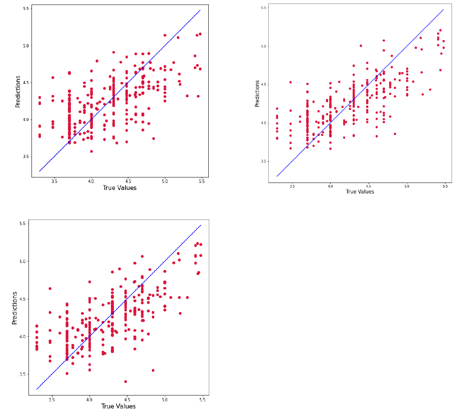
Figure 2: The scatterplots

The K–Nearest Neighbors method The Random Forest method

The Gradient Boosting method

Figure 2 displays the scatterplots of the actual amount of loans and the predicted amount of

loans, based on different machine learning techniques.

7 Conclusion

This paper investigates the factors that explain why households take out informal loans and the

amount of informal loans they take. We use household survey data, which cover around 4,800

households in 12 provinces across Thailand’s six regions. Our analysis consists of two parts. First,

we present stylized facts about informal loans. Around 42.3 percent of individuals have an infor-

mal loan, with the average informal loan equal to 54,300 baht per person.

Second, we investigate the effects of household characteristics on the decision to take an infor-

mal loan and the amount of informal loans. According to a Probit model and a Logit model, the

number of household members, their savings, and the amount of existing formal loans are main

factors. We then use linear models with ﬁxed effects to estimate the effects of household charac-

teristics on the amount of informal loans and ﬁnd that the number of household members and

personal income are main factors.

Third, we compare predictions of borrowing behavior using three machine learning techniques:

K–Nearest Neighbors, Random Forest, and Gradient Boosting. The results suggest that Random

Forest is the best model for classifying data and estimating the amount of informal loans in general.

Gradient Boosting, on the other hand, can provide a classiﬁcation accuracy rate of 76.46 percent if

the model uses only the 15 most important features.

References

[1] Chemin, M. (2008). The beneﬁts and costs of microﬁnance: Evidence from Bangladesh. Journal

of Development Studies, 44(4), 463–484. doi:10.1080/00220380701846735

[2] Dutt, P., & Tsetlin, I. (2020). Income distribution and economic development: Insights from

machine learning. Economics & Politics 33(1), 1–36. https://doi.org/10.1111/ecpo.12157

[3] Guirkinger, C. (2008). Understanding the coexistence of formal and informal credit markets

in Piura, Peru. World Development, 36(8), 1436–1452. doi:10.1016/j.worlddev.2007.07.002

[4] Jeromi, P. D. (2007). Regulation of informal ﬁnancial institutions: A study of money lenders

in Kerala. Reserve Bank of India Occasional Papers, 28(1), 1–32.

[5] Kaboski, J., & Townsend, R. (2005) Policies and impact: An analysis of village-level microﬁ-

nance institutions. Journal of the European Economic Association, 3(1), pp. 1–50.

[6] Kislat, C. (2015), Why are informal loans still a big deal? Evidence from Northeast Thailand.

The Journal of Development Studies, 51(5), 569–585. doi: 10.1080/00220388.2014.983907

[7] Kislat, C., Menkhoff, L., & Neuberger, D. (2017). Credit market structure and collateral in rural

Thailand. Economic Notes, 46, 587–632. doi: 10.1111/ecno.12089

[8] Klühs, T., Koch, M., & Stein, W. (2019). Don’t expect too much: High income expectations and

over-indebtedness. Discussion Paper 200, CRC TRR 190.

[9] Liu, E., & Roth, B. (2020). Contractual restrictions and debt traps.

https://doi.org/10.2139/ssrn.3080682

[10] Mohieldin, M., & Wright, P. W. (2000). Formal and informal credit markets in Egypt. Economic

Development and Cultural Change, 48(3), 657–670. doi: 10.1086/452614

[11] Pitt, M., & Khandker, S. (1998) The impact of group-based credit programs on poor house-

holds in Bangladesh: Does the gender of participants matter? Journal of Political Econ-

omy,106(5), pp. 958–996.

[12] Siamwalla, A., Pinthong, C., Poapongsakorn, N., Satsanguan, P., Nettayarak, P., Mingma-

neenakin, W., & Tubpun, Y. (1990). The Thai rural credit system: Public subsidies, private

information, and segmented markets. The World Bank Economic Review, 4(3), 271–295.

[13] Tanomchat, W., & Sampattavanija, S. (2018). Dependence of informal interest rates and level of

lenders’ inﬂuence in the informal loan market in Thailand. International Advances in Economic

Research, 24(1), 47–63. https://doi.org/10.1007/s11294-018-9672-1

Figure 1: The correlation plot of selected 15 features using dataset 2.