Microsoft Word - SVM-Based Spam Filter with Active and Incremental Learning.doc

SVM-Based Spam Filter with Active and

Online Learning

Qiang Wang Yi Guan Xiaolong Wang

School of Computer Science and Technology, Harbin Institute of Technology, Harbin 150001, China

Email:{qwang, guanyi, wangxl}@insun.hit.edu.cn

Abstract

A realistic classification model for spam filtering should not only take account of the fact that spam evolves

over time, but also that labeling a large number of examples for initial training can be expensive in terms of

both time and money.

This paper address the problem of separating legitimate emails from unsolicited

ones with active and online learning algorithm

, using a Support Vector Machines (SVM) as the base

classifier. We evaluate its effectiveness

using a set of goodness criteria on TREC2006 spam filtering

benchmark datasets, and promising results are reported.

1. Introduction

The well-documented problem of unsolicited email, or spam, is currently of serious and escalating concern.

To date m

ost research in the area of spam detection has focused on some tasks like non-stationarity of

the data source, severe sampling bias in the training data, and non-uniformity of misclassification

costs.

Unfortunately, the researches on spam filtering rarely takes account of the fact that spam should

evolve over time and we should adopt an efficient strategy to accelerate the learning process.

In this paper, we explicitly address the necessity and feasibility of the adaptive learning strategy to

spam filtering task. We present and evaluate a classification model for spam filtering with active and

online learning algorithm. The research focuses on the use of Support Vector Machines (SVMs) as our

base classifier, since their demonstrated robustness and ability to handle large feature spaces makes

them particularly attractive for this task. Based on SVMs, an active learning algorithm that adopts

informative-ness combined with diversity as selection criterion and an online learning strategy that

only use the historical SV samples and the incremental training samples in re-training are studied, and

their performance is evaluated on TREC2006 spam filtering benchmark datasets. Advantages of

directly accounting for active and online learning methods are demonstrated.

In the remainder of this paper, we first give a short survey of related work, and then describe the active

and online algorithm in detail. After that, we present our results of applying the algorithm to email

classification. Finally, we give our conclusions and discuss the prospects for future work.

2. Related Work

The spam filtering problem has traditionally been presented as an instance of a text categorization problem

with the categories being spam and ham. In reality, the structure of email is richer than that of flat text,

with meta-level features such as the fields found in MIME compliant messages. Researchers have recently

acknowledged this, setting the problem in a semi-structured document classification framework. Several

solutions have been proposed to overcome the spam problem. Among the proposed methods, much interest

has focused on the machine learning techniques in spam filtering. They include rule learning

[1]

, Naive

Bayes

[2, 3]

, decision trees

[4]

, support vector machines

[5]

or combinations of different learners

[6]

. The basic

and common concept of these inductive approaches is that using a classifier to filter out spam and the

classifier is learned from training data rather than constructed by hand.

Usually spam filtering task is a continuous work with email sequence increasing in size, there is a need

to scale up the learning algorithms to handle more training data. And since it is time consuming to retrain

the classifier whenever a new example is added to the training set, it is more efficient from a computational

point of view to minimize the number of labeled examples to learn a function at a certain accuracy level.

We can use Support Vector Machines (SVMs) and adopt the active and online learning techniques as

possible solutions to these problems. SVMs have worked well for the incremental model learning

[7, 8]

and

have shown impressive performance in the active learning

[9]

applications for its nice properties of

summarizing data in the form of support vectors.

The active learning is to select the most useful example

for labeling and add the labeled example to training set to retrain model. Tong and Koller

[10]

control the

labeling effort and accelerate the learning process by using the current SVM classifier to query the instance

closest to the decision hyperplane in terms of version space bisection. Brinker

[11]

first incorporate diversity

criterion in active learning

to maximize the training utility of a batch. The online learning is attractive

for solving the problem of dynamic nature of data and drifting concepts.

The elegant solution to online

SVM learning is the incremental SVM which provides a framework for exact online learning.

Syed

[12]

et al.

proposed an incremental SVM learning algorithm, which uses only the historical SV samples and the

incremental training samples in re-training. All non-SV samples are discarded after previous training.

Xiao

[13]

et al. proposed a different incremental learning approach for SVM based on the boosting idea.

hese scalability and accelerative learning task are almost confined to the text classification task and

seldom discussed in spam filtering.

3. Active and Online Learning for Spam Filtering Task

3.1 Brief Introduction of SVM

The main idea of Support Vector Machine is to construct a nonlinear kernel function to map the data

from the input space into a possibly high-dimensional feature space and then generalize the optimal

hyper-plane with maximum margin between the two classes.

Given a T-element training set {(x

):x

∈

∈{-1,1},i=1,…,T} a linear SVM classifier:

()

ii ii

Fx a

xx b x a

xbxwb

⋅+=⋅ +=⋅+

∑∑

(1)

Where a

≥0, b is a bias term and D is the dimension of the input space; · is a dot-product operator,

and w is the normal vector of the classification hyperplane. Typically, the multipliers a

have non-zero

values only for a small subset of the training set, which is called the support set and its elements the

support vectors. The optimal hyperplane is found such as to maximize the classification margin, given

by 2/‖w‖

, where w denotes the normal vector of the hyperplane. The soft-margin optimization task

is formulated as:

min :

: ( ) 1

imize C w

subject to y w x b

⋅

+≥−

∑

(2)

Where C

≥0, p≥0 and ξ

=(1-y(w·x+b));(z)

=z for z≥0 and is equal to 0 otherwise; The slack

variables ξ

take non-zero values only for bound support vectors, i.e., points that are misclassified or

lie inside the classifier’s margin. Note that in eq.(2) the accuracy over the training set is balanced by

the “smoothness” of the solution. We will consider the case of p=1, for which a number of highly

efficient computational methods have been developed.

3.2 Active Learning for Spam Filtering

So far we have considered learning strategies in which data is acquired passively. However, SVMs

construct a hypothesis using a subset of the data containing the most informative patterns and thus

they are good candidates for active or selective sampling techniques which seek out these patterns.

Suppose the data is initially unlabeled, a good heuristic algorithm would predominantly request the

labels for those patterns which will become support vectors. Active selection would be particularly

important for practical situations in which the process of labeling data is expensive or the dataset is

large and unlabeled.

Tong

[10]

proposed the Simple algorithm, which iteratively chooses h unlabeled instances closest to

the separating hyperplane to solicit user feedback. Based on this algorithm, a first spam filter f can be

trained on the labeled email pool L. Then the f is applied to the unlabeled e-mail pool U to compute

each unlabeled e-mail’s distance to the separating hyperplane. The h unlabeled e-mails closest to the

hyperplane and relatively apart are chosen as the next batch of samples for conducting pool-queries.

However, the Simple algorithm may choose too many similar queries, which impairs the learning

performance. We adopted diversity measure presented by Brinker

[11]

to construct batches of new

training examples and enforces selected examples to be diverse with respect to their angles. The main

idea is to select a collection of emails close to the classification hyperplane, while at the same time

maintaining their diversity. The diversity of email is measured by the angles. For example, suppose x

has a normal vector equal to (x

). The angle between two hyperplanes h

and h

, corresponding to the

email instances x

and x

, can be written in terms of the kernel operator K:

The angle-diversity algorithm starts with an initial hyperplane h

trained by the given labeled email

set L. Then, for each unlabeled email x

, it computes the distance to the classification hyperplane h

The angle between the unlabeled x

and the current set S is defined as the maximal angle from x

to any

other x

in set S. This angle measures how diverse the resulting S would be, if x

were to be chosen as a

sample. Algorithm angle-diversity introduces a parameter to balance two components: the distance

from emails to the classification hyperplane and the diversity of angles among different emails.

Incorporating the trade-off factor, the final score for the unlabeled x

can be written as

Where function f computes the distance to the hyperplane, function K is the kernel operator, and S is

the training set. After that, the algorithm selects as the sample the unlabeled email that enjoys the

smallest score in U. The algorithm repeats the above steps h times to select h emails. In practice, the

complete method uses a weighted sum of diversity and hyperplane distance, controlled by a parameter

λ, where λ= 0 is the equivalent of focusing solely on diversity and λ= 1 is the same as Simple. We

determined that λ= 0.5 worked well for our experiments.

3.3 Online Learning for Spam Filtering

Online learning is an important domain in machine learning with interesting theoretical properties and

practical applications. Online learning is performed in a sequence of trials. At trial t the algorithm first

receives an instance x

∈ R

and is required to predict the label associated with that instance. After the

online learning algorithm has predicted the label, the true label is revealed and the algorithm pays a

unit cost if its prediction is wrong. The ultimate goal of the algorithm is to minimize the total number

of prediction mistakes it makes along its run. To achieve this goal, the algorithm may update its

prediction mechanism after each trial so as to be more accurate in later trials.

In this paper, we assume that the prediction of the algorithm at each trial is determined by a SVMs

classifier. Usually in SVMs only a small portion of samples have non-zero

i

coefficients, whose

corresponding x

(support vectors) and y

fully define the decision function. Therefore, the SV set can

fully describe the classification characteristics of the entire training set. Because the training process

of SVM involves solving a quadratic programming problem, the computational complexity of training

process is much higher than a linear complexity. Hence, if we train the SVM on the SV set instead of

the whole training set, the training time can be reduced greatly without much loss of the classification

precision. This is the main idea of online learning algorithm.

Given that only a small fraction of training emails end up as support vectors, the support vector

algorithm is able to summarize the data space in a very concise manner. The training

[12]

would use

only the historical SV samples and the incremental training samples in re-training. All non-SV

samples are discarded after previous training. Figure 1 shows the incremental training procedure.

() ( ) (, )

cos( ( , ))

() ( )

(,)(, )

ij ij

ii i j

xx Kxx

Kx x Kx x

Φ⋅Φ

∠= =

ΦΦ

(3)

(, )

() (1 )(max )

(,)( , )

ii j j

kx x

Kx x Kx x

λλ

∈

⋅+−⋅

(4)

Let us call the training email set as TR, so we trained an initial spam filter on TR. Then we took the

support vectors chosen from TR, called SV

, and classify the instances x

in trial sequence. After

querying the true label of x

, we add x

to SV

if the filter’s prediction is wrong. Again we ran the SVM

training algorithm on SV

+ x

. Now the SVs chosen from the training of SV

+ x

were taken, let us

call these SV

. Again the training and testing were done. This incremental step was repeated until all

the trials are used. The algorithm can be illustrated in algorithm 1 as follows.

The model obtained by this method should be the same or similar to what would have been obtained

using all the data together to train. The reason for this is that the SVMs algorithm will preserve the

essential class boundary information seen so far in a very compact form as support vectors, which

would contribute appropriately to deriving the new concept in the next iteration.

4. Evaluations and Analysis

4.1 Experiment Setting

In this section, we report the test results on four email datasets provided by TREC 2006 spam track.

The basic statistics for all four datasets are given in Table 1.

Ham Spam Total

Trec06p/full

12910 24912 37822

Public Corpora

Trec06c/full

21766 42854 64620

X2 9039 40135 49174

Private Corpora

B2 9274 2751 12025

The experiment is evaluated by a number of criteria that were used for the official evaluation:

• hm%: Ham Misclassification Rate, the fraction of ham messages labeled as spam.

•

sm%: Spam Misclassification Rate, the fraction of spam messages labeled as ham.

• 1-ROCA: Area above the Receiver Operating Characteristic (ROC) curve.

•

Lam%: logistic average misclassification percentage defined as, lam% = logit

-1

(logit(hm%)/2 +

logit(sm%)/2), where logit(x) = log(x/(1-x)) and logit

-1

(x) = e

/(1+e

The spam track includes two approaches to measuring the filter’s learning curve: (1) piecewise

approximation and logistic regression are used to model hm% and sm% as a function of the number of

Online SVM Spam Filter:

1) Initialization

Seed SVM classifier with a few examples of each class (spam and ham)

Train an initial SVM filters

2) Online Learning

- Classify x

- Query the true label of x

- If the filter’s prediction is wrong, retrain SVM filters based on SV

+ x

3) Finishing

Repeat until x

is finished

Table 1. Basic statistics for the evaluation datasets

ure 1. The Incremental Trainin

Procedure

X0 X1 X2 ... Xn

SV2 SV3 SVn-1

Target

Concept1

Target

Concept2

Target

ConceptN-1

Final

Concept

SV1

Trials

Sequence

messages processed; (2) cumulative (1-ROCA)% is given as a function of the number of messages

processed.

4.2 Results

4.2.1 Experiment I: The Impact of Active Learning Method

The first experiment was designed to find whether the active learning strategy perform similarly on

two-class spam filtering task with Multivariate Performance Measures like 1-ROCA in mind. To this

end, the spam filter is first requested to select a sequence of messages from the first 90% of the corpus

as "teach me" examples. That is, the filter is trained on the correct classification for these, and only

these examples. Secondly, from time to time (after 100, 200, 400, etc. "teach me" examples) the filter

is asked to classify the remaining 10% of the corpus, one-at-a-time, in order. The performance of

active selection (AL) and random adding training examples (RL) are compared.

The graphs in Figure 2-3 illustrate the performance of our active and random learning method on

trec06p and trec06c respectively. We can make two useful observations when putting the results

together (Figures 2 to 3). The first thing we notice with the number of training examples increasing we

observed higher generalization accuracy for the active learning strategy and the random strategy in all

our experiments.

This corresponds to the intuition that the more training examples, the more prediction

power a classifier can produce.

The second thing is that active selection can minimize the number of

labeled examples that are necessary to learn a classification function at a certain accuracy level, especially

when

there are comparatively few support vectors to find. In figure 2, there are altogether 34,040

examples to be learned. The AL filter performance promotes very fast that the AL.3200 achieves the

Figure 3. ROC curves for AL (left) and RL (right) filters on the trec06c corpus.

Figure 2. ROC curves for AL (left) and RL (right) filters on the trec06p corpus.

comparable performance with AL.25600. While the RL filter works best until the RL.25600 finished.

In figure 3, same trend is still obviously. There are altogether 58,158 examples to be learned. The best

performance obtained at AL12800 and RL.51200 respectively. Since the difference in performance is

much stable between different datasets as seen in the graphs, we may conclude that the random

selection cannot provide the same level of spam detection provided by the active learning filters.

4.2.2 Experiment II: The Impact of Online Learning Method

This experiment run in a controlled environment simulating personal spam filter use to verify the

online learning performance on the official corpus. The system was first presented a sequence of

messages, one message at a time, and was required to return a “spamminess” score (a real number

representing the estimated likelihood that the message is spam). After that the correct classification

was presented. Two kinds of online learning strategy are tested respectively, the ideal and delayed user

feedback. In ideal user feedback, the filter retrains the model immediately after each classification.

And in the delayed feedback, the filter will not be retained immediately. That is random-sized

sequences of email messages will be classified without any intervening "train" commands and the

corresponding "train" commands for these messages will follow, with no intervening "classify"

commands. The length of the sequences will be randomly generated with an exponential distribution.

A summary of the results achieved with Ideal user feedback (Ideal) against Delayed user feedback

(Delayed) learning algorithm data on the official corpus is listed in the Table 2. Overall, the Ideal

system outperformed the other system on most of the evaluation corpora in the 1-ROCA criterion.

However, the tradeoff between ham misclassification and spam misclassification varies considerably

for different datasets.

Hm% Sm% Lam% 1-ROCA

Ideal Delayed Ideal Delayed Ideal Delayed Ideal Delayed

Trec06p

3.00

(2.71-3.31)

4.44

(4.09-4.81)

0.89

(0.78-1.02)

2.15

(1.97-2.34)

1.64

(1.52-1.77)

3.10

(2.93 -3.28)

0.2884

(0.2479 - 0.3355)

0.5783

(0.5281 - 0.6332)

Trec06c

2.58

(2.37-2.80)

11.29

(10.87-11.72)

0.73

(0.65-0.82)

1.55

(1.43-1.67)

1.38

(1.29 -1.48)

4.28

(4.10 -4.47)

0.2054

(0.1751 - 0.2409)

1.3803

(1.2914 - 1.4753)

2.82

(2.49-3.18)

7.09

(6.57-7.64)

0.47

(0.40-0.54)

1.29

(1.18-1.40)

1.15

(1.05 -1.26)

3.06

(2.89 -3.24)

0.1412

(0.1142 - 0.1747)

0.5184

(0.4611 - 0.5829)

2.18

(1.89-2.50)

2.99

(2.65-3.35)

4.14

(3.43-4.96)

8.83

(7.80-9.96)

3.01

(2.68 -3.38)

5.18

(4.74 -5.65)

0.5806

(0.4829 - 0.6979)

1.2829

(1.1013 - 1.4940)

A comparison with the statistics in Table 2 reveals that our online system disproportionately favored

classification into the class that contains more training examples. The online system did not vary the

filtering threshold dynamically, but rather kept it fixed at a spamminess score. The results indicate that

adjusting the threshold with respect to the number of ham and spam training examples or, alternatively,

with respect to previous performance statistics, would be beneficial.

Table 2. Misclassification Summary

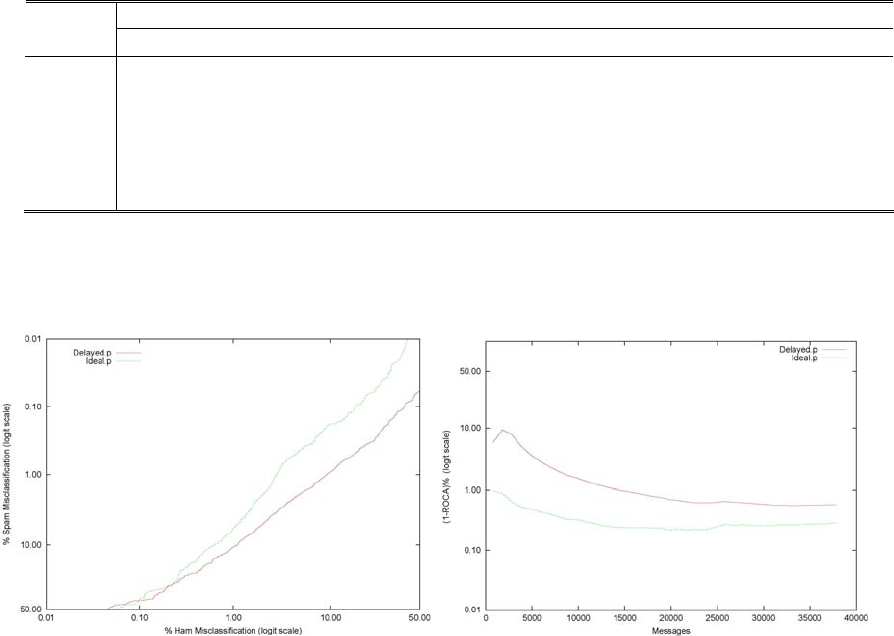
Figure 4. ROC curves (left) and learning curves (right) for Ideal and Delayed filters on trec06p corpus.

The ROC and ROC learning curves for the Ideal and Delay on the trec06p and trec06c result are

depicted in Figure 4-5. The left figures depicts the ROC curve of the Ideal and Delay system, it

provide a convenient graphical display of the trade-off between true and false positive classification

rates for spam filtering task. We can interpret this curve as a comparison of the Ideal filter

performance across the entire range of class distributions and error costs. The performance improves

the further the curve is near to the upper left corner of the plot. The left figures show that the Ideal

system dominates the other curve over most regions. The right graph shows how the area above the

ROC curve changes with an increasing number of examples. The performance improves the further

the curve is near to the lower left corner of the plot. Note that the 1-ROCA statistic is plotted in

log-scale. All filters learn fast at the start, but performance levels off at around 10,000 messages. This

behavior may be attributed to the implicit bias in the learning algorithms, data or concept drift. It

remains to be seen whether a more refined model pruning strategy would help the filter to continue

improving beyond this mark.

5. Conclusions

Our system reached the anticipated goal in the TREC evaluation. The TREC results confirmed our

intuition that active and online learning offer a number of advantages over random selection and

delay-retraining spam filtering methods. By using active learning algorithm, the spam filter can faster

attain a level of generalization accuracy in terms of the number of labeled examples. Also, the online

learning algorithm, whereby only subsets of the data are to be considered at any one time and results

subsequently combined, can make the retraining process much faster and avoid the much storage cost.

Thus the filter algorithm can be scaled up to handle extremely large data sets.

This active and online spam filter achieved the best ranking filter overall in the 1-ROCA statistic for

most of the datasets in the official evaluation. Despite the encouraging results at TREC, we believe

there is much room for improvement in our system. To most users spam is a nuisance, while the loss

of legitimate email is much more serious, so the filter should define an optimal threshold to one that

rejects a maximum amount of spam while passing all legitimate emails. In future work, we intend to

employ a suitable mechanism for dynamically adapting the filtering threshold. And while traditional

SVMs only use the error rate, not the application specific performance measure like ROC-Area, as the

performance measure to optimize model, it is likely to produce suboptimal results. An interesting

avenue for future research would be to employ a strategy which would directly optimize SVMs for

1-ROCA measure that promotes spam filter performance.

Acknowledgements

This research was supported by National Natural Science Foundation of China (60435020, 60504021)

and Key Project of Chinese Ministry of Education & Microsoft Asia Research Centre (01307620).

References

Figure 5. ROC curves (left) and learning curves (right) for Ideal and Delayed filters

on trec06c corpus.

[1] W.W. Cohen. Learning Rules that Classify E-mail. In Proceedings of AAAI Spring Symposium on

Machine Learning in Information Access. USA: 1996. 18-25.

[2] I. Androutsopoulos,J. Koutsias,K.V. Chandrinos,G. Paliouras and C.D. Spyropoulos. An Evaluation of

Naive Bayesian Anti-Spam Filtering. In Proceedings of the Workshop on Machine Learning in the New

Information Age, 11th European Conference on Machine Learning (ECML). Barcelona, Spain: 2000. 9-17.

[3] M. Sahami,S. Dumais,D. Heckerman and E. Horvitz. A Bayesian Approach to Filtering Junk E-Mail.

In Proceedings of AAAI Workshop on Learning for Text Categorization. Isconsin, USA: 1998. 55-62.

[4] X. Carreras and L. Marquez. Boosting Trees for Anti-Spam Email Filtering In Proceedings of Euro.

Conference Recent Advances in NLP (RANLP-2001). Tzigov Chark, Bulgaria.: 2001. 58-64.

[5] A. Kolcz and J. Alspector. SVM-based Filtering of E-mail Spam with Content-specific

Misclassification Costs. In Proceedings of the TextDM'01 Workshop on Text Mining. California, USA: 2001

[6] G. Sakkis,I.Androutsopoulos,G. Paliouras,V.Karkaletsis,C.D. Spyropoulos and P. Stamatopoulos.

Stacking Classifiers for Anti-Spam Filtering of E-mail. In Proceedings of the 6th Conf. on Empirical

Methods in Natural Language Processing. Pittsburgh,USA: 2001. 44-50.

[7] Martin, M., On-Line Support Vector Machines for Function Approximation, in Technical

Report(LSI-02-11-R). 2002, Catalunya: Department of Software, Universitat Politecnica de Catalunya.

[8] Cauwenberghs G and Poggio T. Incremental and Decremental Support Vector. In Advances Neural

Information Processing Systems: 2001. 409-415.

[9] S. Fine and K. Scheinberg. Incremental Learning and Selective Sampling via Parametric

Optimization Framework for SVM. In Advances in Neural Information Processing Systems. Kluwer

Academic: 2002. 705-711.

[10] Simon Tong and Daphne Koller. Support Vector Machine Active Learning with Applications to Text

Classification. The Journal of Machine Learning Research, 2002. Volume 2 45 - 66

[11] Brinker, Klaus. Incorporating Diversity in Active Learning with Support Vector Machines. In The

Twentieth International Conference on Machine Learning (ICML-2003). Washington, DC USA: 2003.

59--66.

[12] Syed, N.,H. Liu and K. K. Sung. Incremental Learning with Support Vector Machines. In Proc.

Workshop on Support Vector Machines at the International Joint Conference on Artificial Intelligence

(IJCAI-99). Stockholm, Sweden: 1999. 352-356.

[13] Xiao R,Wang J and Zhang F. An Approach to Incremental SVM learning algorism. In Proceeding. the

12th International Conference on Tools with Artificial Intelligence: 2000. 268-273.